Work Life Festival 2025 เป็น event ที่จัดขึ้นเมื่อวันที่ 7–8 พฤศจิกายนที่ผ่านมา โดยในงานมีเวทีนำเสนอในหลากหลายหัวข้อที่ตอบโจทย์วัยทำงาน เช่น:
- การเงินการลงทุน
- การทำธุรกิจ
- การพัฒนาทักษะ
- การใช้ชีวิต
ในบทความนี้ ผมจะมาสรุปเนื้อหาจาก 4 sessions ที่น่าสนใจที่ผมมีโอกาสได้ไปร่วมฟัง:
- The Future of Work (กษิดิศ สตางค์มงคล): วิธีการเอาตัวรอดในโลกอนาคต
- Barista FIRE (วิฑูรย์ สูงกิจบูลย์): วิธีการเกษียณก่อนอายุ ทำยังไงให้ทำงานน้อยลงแต่มีรายได้และเวลาเพิ่มขึ้น?
- Income Maximisation Strategy (ศิวกร ปล้องใหม): วิธีเพิ่มรายได้ให้ถึงขีดสุด
- Purpose First, Market Later (ศรารัญย์ คาน): วิธีการลงทุนให้ตอบโจทย์ชีวิต
ถ้าพร้อมแล้ว ไปเริ่มกันเลย
- 🦾 The Future of Work: Why Now Is the Best Time to Build One-Person Business
- 🧧 Barista FIRE: แผนที่สู่อิสระกึ่งเกษียณ ทำงานที่อยากทำ ไม่ใช่เพราะต้องทำ
- 💰 Income Maximisation Strategy: กลยุทธเรียบง่ายเพิ่มรายได้ให้ถึงขีดสุด
- 📊 Purpose First, Market Later: The Three Pillars of Lifelong Investing
- 📃 References
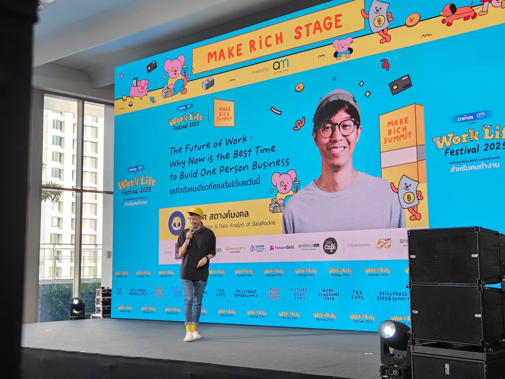
🦾 The Future of Work: Why Now Is the Best Time to Build One-Person Business
Speaker: กษิดิศ สตางค์มงคล (Digital Writer & Data Analyst, DataRockie)
.
🧘 Mindsets for Survival
ไม่มีใครรู้ว่า จะเกิดอะไรขึ้นในอนาคต:
- AI ฉลาดขึ้น
- สิ่งแวดล้อมแย่ลง
- วิกฤตเศรษฐกิจ
- สงครามและความขัดแย้ง
ถ้าจะอยู่รอด เราจะต้องมี mindset 2 ข้อ:
- Accept that everything/reality is just the way it is: ยอมรับในสิ่งที่เป็น ไม่ปฏิเสธหรือต่อต้าน
- No one is coming to save you: ไม่ใครจะช่วยเราได้ (นอกจากตัวเราเอง)
.
🤔 Future Jobs
Job ในอนาคตจะเปลี่ยนจาก job แบบที่พ่อแม่เราทำ (หางานและอยู่กับมันไปนาน ๆ) ไปเป็น job ที่เราสร้างเอง นั่นคือ การสร้างธุรกิจเป็นของตัวเอง (one-person business)
งาน office มีข้อเสียอยู่ 2 ข้อ:
- Less secure: แม้จะดูมั่นคง แต่ก็ไม่เสมอไป หลายองค์กร lay off พนักงาน ทั้งตอน COVID-19 และเมื่อ AI เริ่มเข้ามาแทนที่คน ไม่มีอะไรการันตีว่า เราจะอยู่กับงานที่ทำไปจนเกษียณ
- Effort ≠ reward: ไม่ว่าเราจะทุ่มเทให้กับงานขนาดไหน แต่ไม่มีอะไรการันตีว่า เงินเดือนของเราจะสูงขึ้นตามไป เช่น เราให้เวลากับงานในปีนี้เป็น 2 เท่า แต่ในปีหน้า เราอาจไม่ได้รับเงินเดือนเพราะเศรษฐกิจไม่ดี และเราจะโชคดีมากที่ไม่ถูก lay off
ในทางกลับกัน การมีธุรกิจเป็นของตัวเองมีข้อดี 2 ข้อ:
- More secure: แม้จะไม่มั่นคง 100% แต่ตราบใดที่เรายังสามารถส่งมอบ value ให้กับโลกได้ เราจะสามารถสร้างรายได้อย่างต่อเนื่องและไม่ต้องกลัวตกงาน
- More control: เราควบคุมผลลัพธ์ได้มากกว่า เช่น สร้างรายได้เป็น 2 เท่าจากความพยายามที่เพิ่มขึ้น 2 เท่า
.
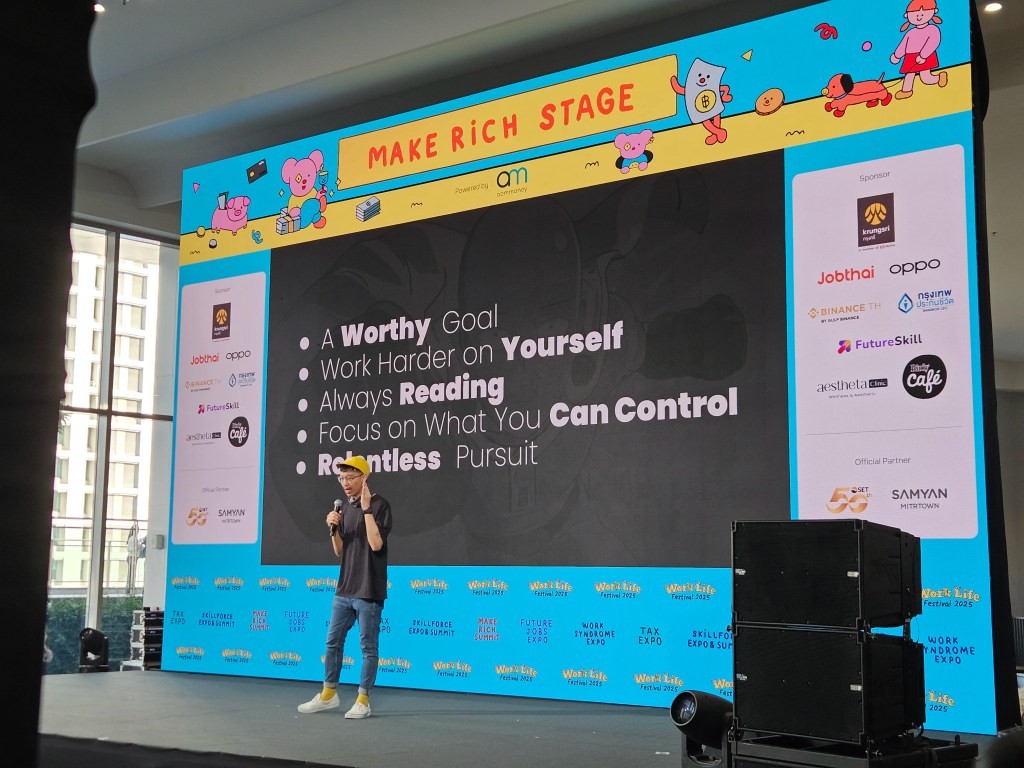
🏦 First-Principles for One-Person Business
เรามีหลักคิด 5 ข้อในการสร้างธุรกิจเป็นของตัวเอง:
- Worthy goal: มองหาเป้าหมายที่คุ้มค่าที่จะลอง
- Work harder on yourself (than on your job): ทุ่มเทไปกับการพัฒนา/ดูแลตัวเอง มากกว่าทุ่มเทให้กับงานที่ทำ (แนวคิดจาก Jim Rohn นักธุรกิจและนักเขียนชาวอเมริกัน)
- Always read: จงอ่านอยู่เสมอ เพราะการเรียนคือชีวิต ไม่ใช่การเตรียมตัวเพื่อใช้ชีวิต (อิงจาก quote ของ John Dewey นักปรัชญาและนักจิตวิทยาชาวอเมริกัน)
- Focus on what you can control: โฟกัสกับสิ่งที่เราควบคุมได้ เพราะสิ่งเดียวที่ไม่มีใครเอาไปจากเราได้ คือ อิสระในการเลือกของเรา (แนวคิดจาก Viktor Frankl นักจิตวิทยาชาวออสเตรียและผุ้รอดชีวิตจากค่ายกักกันของนาซี)
- Relentless pursuit: ทำทุกวัน ทำอย่างสม่ำเสมอ ทำวันละเล็กละน้อยสะสมไป เช่น ถ้าเราอ่านหนังสือเดือนละเล่ม ใน 10 ปีข้างหน้า เราจะมีความรู้เพิ่มขึ้นขนาดไหน
.
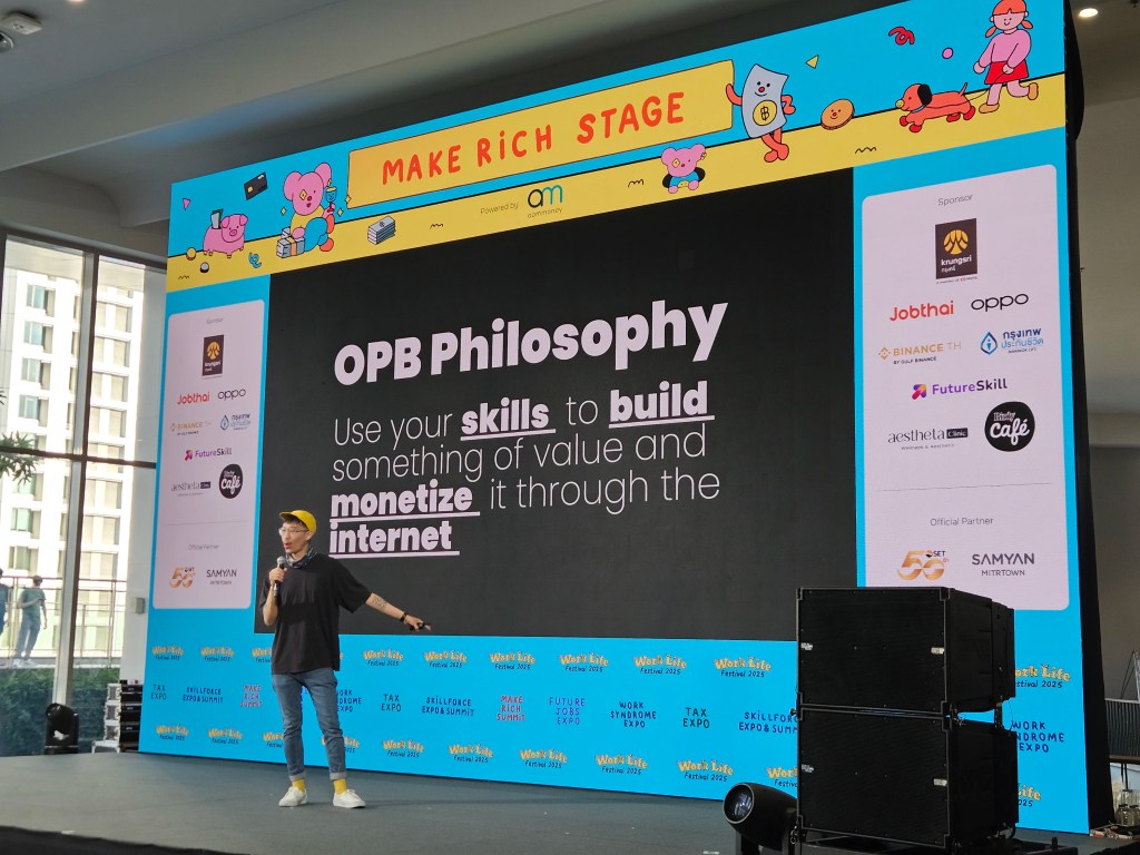
🧑💼 One-Person Business Philosophy
Key takeaway สำหรับการสร้างธุรกิจเป็นของตัวเอง คือ:
Use your skills to build something of value and monetise it through the internet.
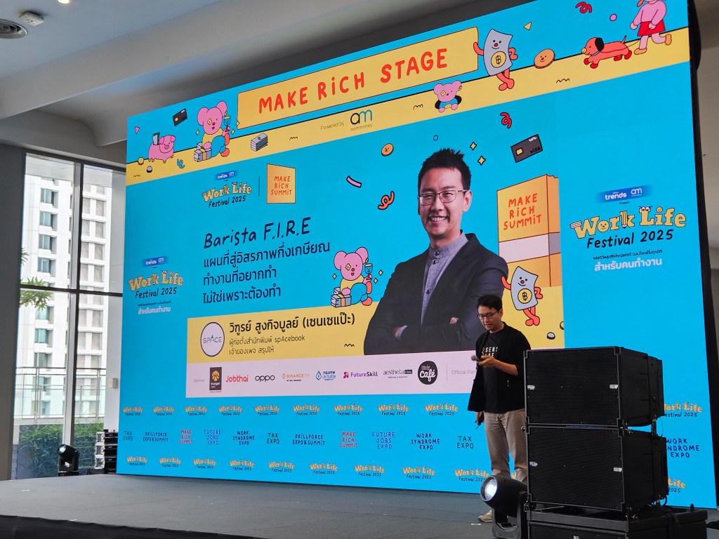
🧧 Barista FIRE: แผนที่สู่อิสระกึ่งเกษียณ ทำงานที่อยากทำ ไม่ใช่เพราะต้องทำ
Speaker: วิฑูรย์ สูงกิจบูลย์ (ผู้ก่อตั้งสำนักพิมพ์ spAcebook, เจ้าของเพจ สรุปให้)
.
📖 Backstory
เมื่อ 10 ปีก่อน คุณวิฑูรย์เคยทำงานเป็นผู้บริหารเงินเดือน 6 หลักและมีชีวิตที่เพียบพร้อม ทั้งเงิน บ้าน รถ และครอบครัว
แต่สิ่งที่ขาดไป คือ ความสุข
คุณวิฑูรย์มีทุกอย่าง แต่ไม่มีเวลาให้กับครอบครัว คุณวิฑูรย์และภรรยาต่างก็เป็นผู้บริหารที่ทำงานหนักด้วยกันทั้งคู่ คุณวิฑูรย์ทำงานหนักจนกระทั่งว่า ลูกคนหนึ่งจะต้องไปอยู่กับยาย/ย่า เพราะทั้งคุณวิฑูรย์และภรรยาไม่มีที่เลี้ยงดูลูกได้อย่างเต็มที่
ทางเลือกของคุณวิฑูรย์มีอยู่ 2 ทาง:
- มีทุกอย่าง แต่ไม่มีเวลาให้กับลูก
- ทำงานน้อยลง แต่มีเวลาให้กับลูก
แน่นอนว่า คุณวิฑูรย์เลือกทางเลือกที่ 2
คุณวิฑูรย์ไม่ได้ออกจากงานในทันที แต่ก็ไม่ได้แผนที่ชัดเจนตอนออกจากงาน
14 งาน คือ งานที่คุณวิฑูรย์ทดลองทำหลังออกจากงาน ตั้งแต่งานแปลเอกสารไปจนถึงขายของในตลาดนัด
ทางเดินของคุณวิฑูรย์ไม่ได้โรยด้วยกลีบกุหลาบ และในวันนี้ คุณวิฑูรย์จะมาแชร์แนวคิดการที่ช่วยให้ทุกคนสามารถทำงานน้อยลง แต่มีรายได้เท่าเดิมหรือมากขึ้น และมีเวลาให้กับชีวิตมากขึ้น
.
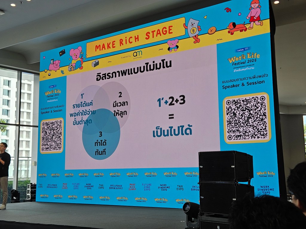
🔥 FIRE & Barista FIRE
แนวคิดที่ว่า คือ FIRE (financial independence, retire early) ซึ่งเป็นวิธีสร้างอิสระทางการเงินด้วยการเก็บออมเงินในขณะที่ยังทำงานอยู่ เพื่อให้สามารถเกษียณตอนอายุยังน้อยและยังมีเงินใช้จ่ายโดยไม่ต้องทำงานอีก
Barista FIRE เป็น FIRE ที่ลดความเข้มข้นในการเก็บออมลงมา โดยแทนที่เราจะออมให้ได้มากพอที่จะสำหรับค่าใช้จ่ายหลังเกษียณ เราจะเก็บเงินแค่ให้มากสำหรับใช้จ่ายบางส่วน และหารายได้เสริมเพื่อดูแลค่าใช้จ่ายที่เหลือ
.
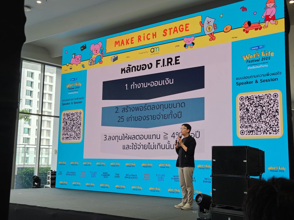
🪜 How to Barista FIRE
การออมแบบ barista FIRE มีอยู่ 3 ขั้นตอน ดังนี้:
- ออม: เก็บเงินในระหว่างที่ยังทำงานประจำอยู่
- ลงทุน: เอาเงินออมไปลงทุนให้ได้ port ขนาด 25 เท่าของค่าใช้จ่ายต่อปี เพื่อให้มี passive income 4% ของค่าใช้จ่ายหลังเกษียณ
- เกษียณ: ออกจากงาน ใช้งานด้วย passive income + ทำงานเสริม
.
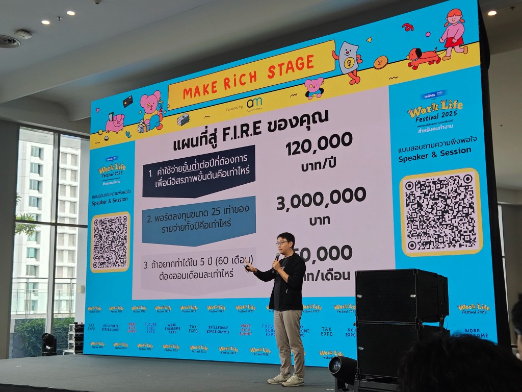
☕ Example
ตัวอย่างการออมเงินให้พอสำหรับเกษียณ:
ถ้าเรามีค่าใช้จ่าย 120,000 บาทต่อปี เราจะต้องสร้าง port ให้ได้ขนาด:
12,000 * 25 = 3,000,000 บาท
และเราต้องการทำ port ให้ได้ภายใน 5 ปี (60 เดือน) เราจะต้องเก็บเงินเดือนละ:
3,000,000 / 60 = 50,000 บาท
.
🙋 Start With This Question
Barista FIRE เป็นแนวทางที่จะช่วยให้เรามีอิสระในการใช้ชีวิตมากขึ้น ซึ่งเราสามารถเริ่มได้ด้วยการถามตัวเองว่า:
เงินขั้นต่ำที่ทำให้เราอยู่ได้โดยไม่เดือดร้อน คือ เท่าไร?
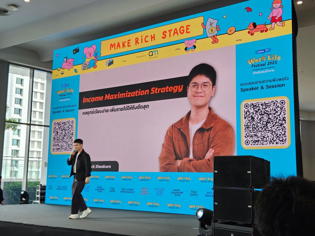
💰 Income Maximisation Strategy: กลยุทธเรียบง่ายเพิ่มรายได้ให้ถึงขีดสุด
Speaker: ศิวกร ปล้องใหม (Founder of Nack Siwakorn)
.
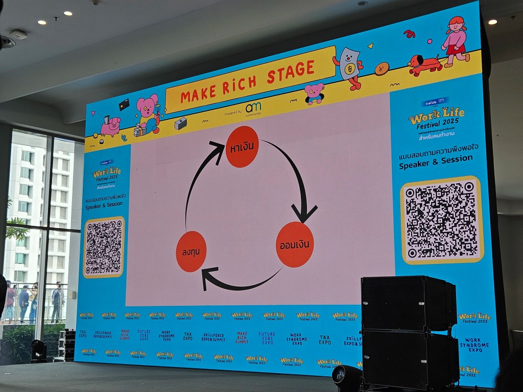
🚲 The Three Wheels of Income
รายได้มาจาก 3 ทาง:
- หาเงิน
- ออมเงิน
- ลงทุน
แต่ละทางเป็นเหมือนล้อจักรยานที่เราต้องออกแรงปั่นเพื่อให้จักรยานเคลื่อนไปข้างหน้า ในช่วงแรก เราจะต้องออกเยอะหน่อย แต่เมื่อล้อหมุนเองได้แล้ว เราจะออกแรงน้อยลงและมีเวลาพักจากการปั่นจักรยานมากขึ้น
.
🚴 How to Move the Wheel
ใน 3 ทางนี้ ทางที่สำคัญที่สุด คือ หาเงิน
ถ้าเรามีเงินทุนเยอะ เราจะสามารถออมและลงทุนได้มากขึ้น นั่นคือ วงล้อการเงินของเราจะหมุนได้ง่ายขึ้น
เราสามารถเพิ่มรายได้ด้วย 2 วิธี:
- เพิ่มรายได้ที่มีอยู่
- หารายได้เสริม
.
🔥 Expand Existing Income
การหาเงินไม่มีอยู่จริง เราไม่สามารถมองหาเงินและเจอเงินล้านตกอยู่บนพื้นได้
ถ้าเราต้องการหาเงิน สิ่งที่เราต้องมองหาไม่เงิน แต่คือปัญหา
ถ้าเราสามารถแก้ปัญหาให้กับกลุ่มคนที่ต้องการทางออกได้ เราก็จะได้เงินที่เรามองหา
การทำงานทุกอย่างคือการแก้ปัญหา เช่น การติว IELTS คือการแก้ปัญหาการสอบเข้ามหาวิทยาลัยให้กับนักเรียนม.ปลาย
เราสามารถเพิ่มรายได้ที่มีอยู่ได้ 2 ทาง:
- แก้ปัญหาที่ใหญ่ขึ้น: เช่น สอน IELTS ให้พนักงานที่ต้องการทำงานในองค์กรต่างชาติ ซึ่งมีกำลังจ่ายมากกว่านักเรียนม.ปลาย
- แก้ปัญหาให้คนมากขึ้น: เช่น เปลี่ยนการสอนแบบตัวต่อตัว เป็นสอนแบบกลุ่ม
.
⌨️ Find Extra Income
อีกวิธีในการเพิ่มรายได้ คือ ทำงานเสริม
งานเสริมที่เราสามารถทำได้ เช่น:
- Video editor
- Graphic designer
- Content creator
- Fitness coach
- Financial advisor
- Tutor
- Consultant
- Seller
- อื่น ๆ
หลายคนอาจมีคำถามเกี่ยวการเริ่มทำงานเสริม เช่น:
- ไม่รู้จะทำอะไร
- ทำไม่เป็น
- ไม่มีทุน
- ไม่มี passion
แต่ทุกคำถามมีคำตอบ:
- ไม่รู้จะทำอะไร → ออกไปหา ไปทดลองเพื่อให้รู้ว่าอยากทำอะไร
- ทำไม่เป็น → เราแค่ต้องฝึกฝนเพิ่ม
- ไม่มีทุน → เราสามารถเก็บเงินเพื่อสร้างทุน หรือเริ่มทำในสิ่งที่ไม่ต้องใช้เงินก่อนได้
- ไม่มี passion → เราไม่มี passion เพราะเราทำได้ไม่ดี และเราทำได้ไม่ดีเพราะยังไม่ได้ลองทำ ดังนั้น ทางออกคือเริ่มลงมือทำ
เราไม่จำเป็นต้องพร้อม 100% ก่อนจะเริ่ม เราสามารถเริ่มได้โดย focus ที่ 4 อย่างนี้:
- Now: ทำในสิ่งที่เราสามารถทำได้ทันที
- Doable: ทำสิ่งที่ฝึกฝนได้/มีคนทำอยู่จริง
- Not too demanding: ไม่ใช่สิ่งที่หนักเกินไป/เราแบ่งเวลาให้ได้
- All in later: ค่อย ๆ เริ่มทีละเล็กละน้อย และเมื่อเริ่มไปได้ดี ค่อยทุ่มเต็มที่ 100%
เราจะเริ่มงานเสริมได้ แค่ต้องมี 3 สิ่งนี้:
- เครื่องมือ (เช่น แล็ปท็อป)
- ทักษะ
- แนวทาง (ถ้าเป็นสิ่งที่มีคนเคยทำแล้ว ให้เราเรียนรู้จากคนเหล่านี้)
Pro tip: สิ่งที่สำคัญสำหรับคนที่เริ่มต้นใหม่ ๆ คือการบริหารเวลา ในช่วงแรกที่เรายังทำได้ไม่ดี/ไม่คล่อง เวลาส่วนตัวของเราอาจจะถูกรบกวนบ่อยครั้ง เราจะต้องจัดการเวลาให้ดี จนกว่าทุกอย่างจะเข้าที่เข้าทาง เพื่อให้เรายังมีคุณภาพชีวิตที่ดี
📊 Purpose First, Market Later: The Three Pillars of Lifelong Investing
Speaker: ศรารัญย์ คาน (Investor & Content Creator, Earthh Evans)
.
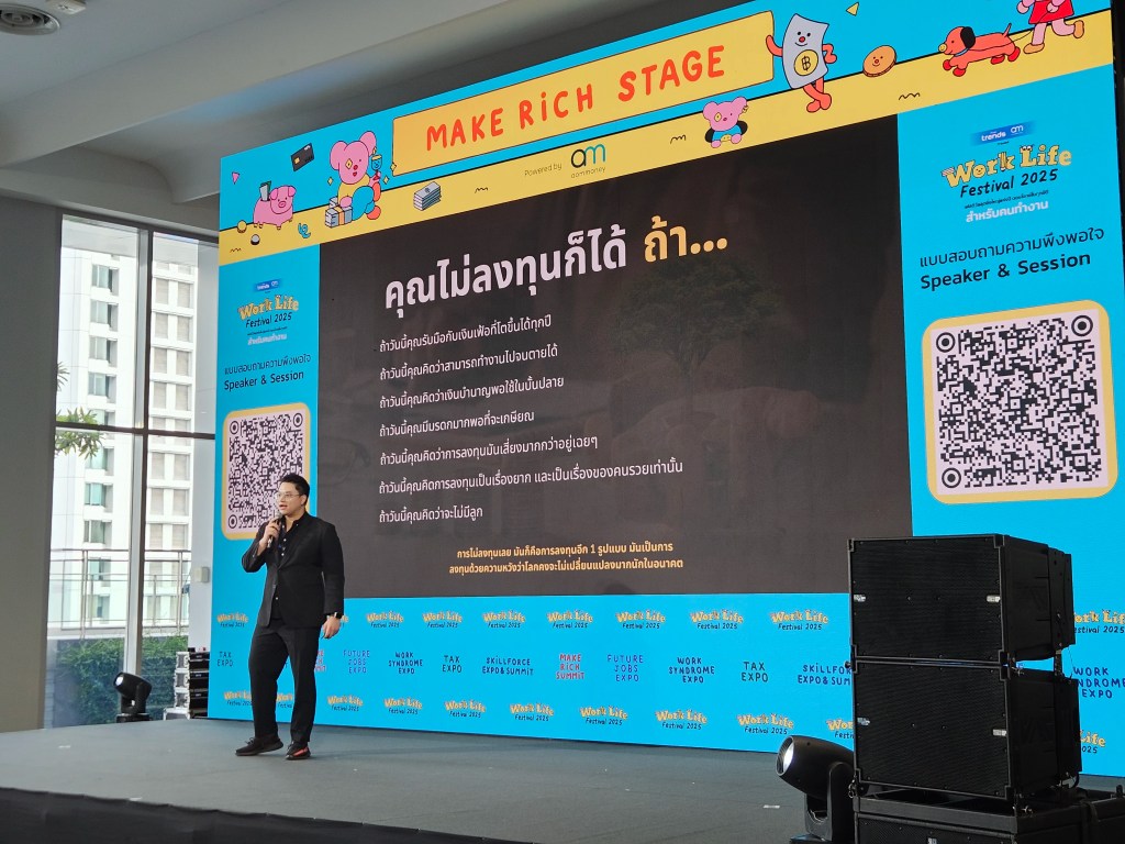
💸 Investing Not Required, Or Not?
กรลงทุนเป็นแค่เครื่องมือ และเราไม่จำเป็นต้องลงทุนก็ได้ถ้า:
- รับมือกับเงินเฟ้อที่เพิ่มขึ้นทุกปีได้
- คิดว่าเราสามารถทำงานไปจนตายได้
- มีเงินพอใช้หลังเกษียณ
- คิดว่าการลงทุนมีความเสี่ยงเกินกว่าที่จะรับได้
- คิดว่าการลงทุนเป็นเรื่องยาก
- ไม่คิดจะมีลูก
จะเห็นว่า หลาย ๆ ข้อเราอาจจะยอมรับ/จัดการไม่ได้ ซึ่งหมายความว่า การลงทุนเป็นสิ่งจำเป็นที่จะช่วยให้เราอยู่รอดได้
.
💖 Put Purpose First
การตัดสินใจว่าจะลงทุนกับอะไร กับตลาดไหน และเท่าไร ขึ้นอยู่กับปัจจัย 3 อย่าง:
- Goal: ไม่ว่าจะเลือกว่าจะลงทุนในสินทรัพย์อะไร ไม่ว่าจะเป็นตลาดไทยหรือต่างประเทศ ทุกอย่างขึ้นกับเป้าหมายของแต่ละคนว่าต้องการมีเงินไปเพื่ออะไร
- Comfort: ความสบายใจต่อปัจจัยต่าง ๆ ที่เกี่ยวข้อง เช่น:
- ภาษีที่มากับการลงทุน
- ค่าธรรมเนียม
- ความผันผวนของค่าเงิน (เช่น อัตราแลกเปลี่ยน)
- ความต่างของเวลาตลาด
- ข่าวสารต่าง ๆ
- Understanding: ความเข้าใจในการลงทุน เช่น:
- ความเข้าใจในธุรกิจ
- ตัวขับเคลื่อนมูลค่า
- โครงสร้างอุตสาหกรรม
- ความเสี่ยงเฉพาะธุรกิจ
.
🪙 Compound Interest
ในการลงทุน เราจะใช้ concept ที่เรียกว่า compound interest หรือดอกเบี้ยทบต้น เพื่อทำเงินให้เรา
เพื่อจะทำให้เราได้ผลตอบแทนที่ดีที่สุดจาก compound interest เราจะต้องพิจารณา 3 อย่าง:
- Capital: เงินต้นที่มากพอ
- Time: เวลาที่มากพอ
- Interest: ผลตอบแทนที่มากพอ
.
📘 Free Investment Playbooks
สำหรับคนที่สนใจเริ่ทต้นลงทุน สามารถโหลด playbooks ความรู้ในการลงทุนได้ฟรีบนโพสต์ของ Earthh Evans
📃 References
- รูปปกบทความจาก ประชาชาติธุรกิจ