วิธีสร้าง linear regression ด้วย lm() ในภาษา R — ตัวอย่างการทำนายราคาเพชรใน diamonds dataset

Written by

Linear regression เป็นวิธีการทำนายข้อมูลด้วยสมการเส้นตรง:

y = a + bx

y = ตัวแปรตาม หรือข้อมูลที่ต้องการทำนาย
a = จุดตัดระหว่าง x และ y (intercept)
b = ค่าความชัด (slope)
x = ตัวแปรต้น

เนื่องจากเป็นเทคนิคที่ใช้งานและทำความเข้าใจได้ง่าย linear regression จึงเป็นวิธีที่นิยมใช้ในการทำนายข้อมูลในบริบทต่าง ๆ เช่น:

ทำนาย	จาก
กำไร	ค่าโฆษณา
ความสามารถของนักกีฬา	ชั่วโมงฝึกซ้อม
ความดันเลือด	ปริมาณยา + อายุ
ผลลิตทางการเกษตร	ปริมาณน้ำ + ปุ๋ย

ในบทความนี้ เราจะมาดูวิธีใช้ linear regression ในภาษา R กัน

ถ้าพร้อมแล้ว ไปเริ่มกันเลย

💎 Example Dataset: diamonds

ในบทความนี้ เราจะใช้ diamonds dataset เป็นตัวอย่างในการใช้ linear regression กัน

diamonds dataset เป็น built-in dataset จาก ggplot2 package ซึ่งมีข้อมูลเพชรมากกว่า 50,000 ตัวอย่าง และประกอบด้วย 10 columns ดังนี้:

No.	Column	Description
1	`price`	ราคา (ดอลล่าร์สหรัฐฯ)
2	`caret`	น้ำหนัก
3	`cut`	คุณภาพ
4	`color`	สี
5	`clarity`	ความใสของเพชร
6	`x`	ความยาว
7	`y`	ความกว้าง
8	`z`	ความลึก
9	`depth`	สัดส่วนความลึก
10	`table`	สัดส่วนความกว้างของยอดเพชรต่อส่วนที่กว้างที่สุด

เป้าหมายของเรา คือ ทำนายราคาเพชร (price)

⬇️ Load diamonds

ในการใช้งาน diamonds เราสามารถเรียกใช้งาน dataset ได้ดังนี้:

ขั้นที่ 1. ติดตั้งและโหลด ggplot2:

# Install
install.packages("ggplot2")

# Load
library(ggplot2)

ขั้นที่ 2. โหลด diamonds dataset:

# Load dataset
data(diamonds)

ขั้นที่ 3. ดูตัวอย่างข้อมูล 10 rows แรกใน dataset:

# Preview the dataset
head(diamonds, 10)

ผลลัพธ์:

# A tibble: 10 × 10
   carat cut       color clarity depth table price     x     y     z
   <dbl> <ord>     <ord> <ord>   <dbl> <dbl> <int> <dbl> <dbl> <dbl>
 1  0.23 Ideal     E     SI2      61.5    55   326  3.95  3.98  2.43
 2  0.21 Premium   E     SI1      59.8    61   326  3.89  3.84  2.31
 3  0.23 Good      E     VS1      56.9    65   327  4.05  4.07  2.31
 4  0.29 Premium   I     VS2      62.4    58   334  4.2   4.23  2.63
 5  0.31 Good      J     SI2      63.3    58   335  4.34  4.35  2.75
 6  0.24 Very Good J     VVS2     62.8    57   336  3.94  3.96  2.48
 7  0.24 Very Good I     VVS1     62.3    57   336  3.95  3.98  2.47
 8  0.26 Very Good H     SI1      61.9    55   337  4.07  4.11  2.53
 9  0.22 Fair      E     VS2      65.1    61   337  3.87  3.78  2.49
10  0.23 Very Good H     VS1      59.4    61   338  4     4.05  2.39

🍳 Prepare the Dataset

ก่อนจะทำนายราคาเพชรด้วย linear regression เราจะเตรียม diamonds dataset ใน 3 ขั้นตอนก่อน ได้แก่:

One-hot encoding
Log transformation
Split data

🪆 Step 1. One-Hot Encoding

ในกรณีที่ตัวแปรต้นที่เป็น categorical เราจะต้องแปลงตัวแปรเหล่านี้ให้เป็น numeric ก่อน ซึ่งเราสามารถทำได้ด้วย one-hot encoding ดังตัวอย่าง:

ก่อน one-hot encoding:

Data	Cut
1	Ideal
2	Good
3	Fair

หลัง one-hot encoding:

Data	Cut_Ideal	Cut_Good	Cut_Fair
1	1	0	0
2	0	1	0
3	0	0	1

ในภาษา R เราสามารถทำ one-hot encoding ได้ด้วย model.matrix() ดังนี้:

# Set option for one-hot encoding
options(contrasts = c("contr.treatment",
                      "contr.treatment"))

# One-hot encode
cat_dum <- model.matrix(~ cut + color + clarity - 1,
                        data = diamonds)

จากนั้น เราจะนำผลลัพธ์ที่ได้ไปรวมกับตัวแปรตามและตัวแปรต้นที่เป็น numeric:

# Combine one-hot-encoded categorical and numeric variables
dm <- cbind(diamonds[, c("carat",
                         "depth",
                         "table",
                         "x",
                         "y",
                         "z")],
            cat_dum,
            price = diamonds$price)

เราสามารถเช็กผลลัพธ์ของ one-hot encoding ได้ด้วย str():

# Check the results
str(dm)

ผลลัพธ์:

'data.frame':	53940 obs. of  25 variables:
 $ carat       : num  0.23 0.21 0.23 0.29 0.31 0.24 0.24 0.26 0.22 0.23 ...
 $ depth       : num  61.5 59.8 56.9 62.4 63.3 62.8 62.3 61.9 65.1 59.4 ...
 $ table       : num  55 61 65 58 58 57 57 55 61 61 ...
 $ x           : num  3.95 3.89 4.05 4.2 4.34 3.94 3.95 4.07 3.87 4 ...
 $ y           : num  3.98 3.84 4.07 4.23 4.35 3.96 3.98 4.11 3.78 4.05 ...
 $ z           : num  2.43 2.31 2.31 2.63 2.75 2.48 2.47 2.53 2.49 2.39 ...
 $ cutFair     : num  0 0 0 0 0 0 0 0 1 0 ...
 $ cutGood     : num  0 0 1 0 1 0 0 0 0 0 ...
 $ cutVery Good: num  0 0 0 0 0 1 1 1 0 1 ...
 $ cutPremium  : num  0 1 0 1 0 0 0 0 0 0 ...
 $ cutIdeal    : num  1 0 0 0 0 0 0 0 0 0 ...
 $ colorE      : num  1 1 1 0 0 0 0 0 1 0 ...
 $ colorF      : num  0 0 0 0 0 0 0 0 0 0 ...
 $ colorG      : num  0 0 0 0 0 0 0 0 0 0 ...
 $ colorH      : num  0 0 0 0 0 0 0 1 0 1 ...
 $ colorI      : num  0 0 0 1 0 0 1 0 0 0 ...
 $ colorJ      : num  0 0 0 0 1 1 0 0 0 0 ...
 $ claritySI2  : num  1 0 0 0 1 0 0 0 0 0 ...
 $ claritySI1  : num  0 1 0 0 0 0 0 1 0 0 ...
 $ clarityVS2  : num  0 0 0 1 0 0 0 0 1 0 ...
 $ clarityVS1  : num  0 0 1 0 0 0 0 0 0 1 ...
 $ clarityVVS2 : num  0 0 0 0 0 1 0 0 0 0 ...
 $ clarityVVS1 : num  0 0 0 0 0 0 1 0 0 0 ...
 $ clarityIF   : num  0 0 0 0 0 0 0 0 0 0 ...
 $ price_log   : num  5.79 5.79 5.79 5.81 5.81 ...

ตอนนี้ ตัวแปรต้นที่เป็น categorical ถูกแปลงเป็น numeric ทั้งหมดแล้ว

📈 Step 2. Log Transformation

ในกรณีที่ตัวแปรตามมีการกระจายตัว (distribution) ไม่ปกติ linear regression ทำนายข้อมูลได้ไม่เต็มประสิทธิภาพนัก

เราสามารถตรวจสอบการกระจายตัวของตัวแปรตามได้ด้วย ggplot():

# Check the distribution of `price`
ggplot(dm,
       aes(x = price)) +
  
  ## Instantiate a histogram
  geom_histogram(binwidth = 100,
                 fill = "skyblue3") +
  
  ## Add text elements
  labs(title = "Distribution of Price",
       x = "Price",
       y = "Count") +
  
  ## Set theme to minimal
  theme_minimal()

ผลลัพธ์:

จากกราฟ เราจะเห็นได้ว่า ตัวแปรตามมีการกระจายตัวแบบเบ้ขวา (right-skewed)

ดังนั้น ก่อนจะใช้ linear regression เราจะต้องแปรตัวแปรตามให้มีการกระจายตัวแบบปกติ (normal distribution) ก่อน ซึ่งเราสามารถทำได้ด้วย log transformation ดังนี้:

# Log-transform `price`
dm$price_log <- log(dm$price)

# Drop `price`
dm$price <- NULL

หลัง log transformation เราสามารถเช็กการกระจายตัวด้วย ggplot() อีกครั้ง:

# Check the distribution of logged `price`
ggplot(dm,
       aes(x = price_log)) +
  
  ## Instantiate a histogram
  geom_histogram(fill = "skyblue3") +
  
  ## Add text elements
  labs(title = "Distribution of Price After Log Transformation",
       x = "Price (Logged)",
       y = "Count") +
  
  ## Set theme to minimal
  theme_minimal()

ผลลัพธ์:

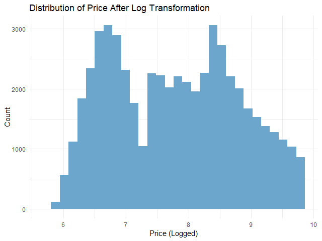
จะเห็นได้ว่า การกระจายตัวของตัวแปรตามใกล้เคียงกับการกระจายตัวแบบปกติมากขึ้นแล้ว

🚄 Step 3. Split the Data

ในขั้นสุดท้ายก่อนใช้ linear regression เราจะแบ่งข้อมูลออกเป็น 2 ชุด:

Training set สำหรับสร้าง linear regression model
Test set สำหรับประเมินความสามารถของ linear regression model

ในบทความนี้ เราจะแบ่ง 80% ของ dataset เป็น training set และ 20% เป็น test set:

# Split the data

## Set seed for reproducibility
set.seed(181)

## Training index
train_index <- sample(nrow(dm),
                      0.8 * nrow(dm))

## Create training set
train_set <- dm[train_index, ]

## Create test set
test_set <- dm[-train_index, ]

ตอนนี้ เราพร้อมที่จะสร้าง linear regression model กันแล้ว

🏷️ Linear Regression Modelling

การสร้าง linear regression model มีอยู่ 3 ขั้นตอน ได้แก่:

Fit the model
Make predictions
Evaluate the model performance

💪 Step 1. Fit the Model

ในขั้นแรก เราจะสร้าง model ด้วย lm() ซึ่งต้องการ input 2 อย่าง:

lm(formula, data)

formula = สูตรการทำนาย โดยเราต้องกำหนดตัวแปรต้นและตัวแปรตาม
data = ชุดข้อมูลที่ใช้สร้าง model

ในการทำนายราคาเพชร เราจะใช้ lm() แบบนี้:

# Fit the model
linear_reg <- lm(price_log ~ .,
                 data = train_set)

อธิบาย code:

price_log ~ . หมายถึง ทำนายราคา (price_log) ด้วยตัวแปรต้นทั้งหมด (.)
data = train_set หมายถึง เรากำหนดชุดข้อมูลที่ใช้เป็น training set

เราสามารถดูข้อมูลของ model ได้ด้วย summary():

# View the model
summary(linear_reg)

ผลลัพธ์:

Call:
lm(formula = price_log ~ ., data = train_set)

Residuals:
    Min      1Q  Median      3Q     Max 
-2.2093 -0.0930  0.0019  0.0916  9.8935 

Coefficients: (1 not defined because of singularities)
                 Estimate Std. Error  t value Pr(>|t|)    
(Intercept)    -2.7959573  0.0705854  -39.611  < 2e-16 ***
carat          -0.5270039  0.0086582  -60.867  < 2e-16 ***
depth           0.0512357  0.0008077   63.437  < 2e-16 ***
table           0.0090154  0.0005249   17.175  < 2e-16 ***
x               1.1374016  0.0055578  204.651  < 2e-16 ***
y               0.0290584  0.0031345    9.271  < 2e-16 ***
z               0.0340298  0.0054896    6.199 5.73e-10 ***
cutFair        -0.1528658  0.0060005  -25.476  < 2e-16 ***
cutGood        -0.0639105  0.0036547  -17.487  < 2e-16 ***
`cutVery Good` -0.0313800  0.0025724  -12.199  < 2e-16 ***
cutPremium     -0.0451760  0.0026362  -17.137  < 2e-16 ***
cutIdeal               NA         NA       NA       NA    
colorE         -0.0573940  0.0032281  -17.779  < 2e-16 ***
colorF         -0.0892633  0.0032654  -27.336  < 2e-16 ***
colorG         -0.1573861  0.0032031  -49.136  < 2e-16 ***
colorH         -0.2592763  0.0034037  -76.175  < 2e-16 ***
colorI         -0.3864526  0.0038360 -100.742  < 2e-16 ***
colorJ         -0.5258789  0.0047183 -111.455  < 2e-16 ***
claritySI2      0.4431577  0.0079170   55.976  < 2e-16 ***
claritySI1      0.6087513  0.0078819   77.234  < 2e-16 ***
clarityVS2      0.7523161  0.0079211   94.976  < 2e-16 ***
clarityVS1      0.8200656  0.0080463  101.918  < 2e-16 ***
clarityVVS2     0.9381319  0.0082836  113.252  < 2e-16 ***
clarityVVS1     1.0033931  0.0085098  117.910  < 2e-16 ***
clarityIF       1.0898015  0.0092139  118.277  < 2e-16 ***
---
Signif. codes:  0 ‘***’ 0.001 ‘**’ 0.01 ‘*’ 0.05 ‘.’ 0.1 ‘ ’ 1

Residual standard error: 0.1825 on 43128 degrees of freedom
Multiple R-squared:  0.9677,	Adjusted R-squared:  0.9676 
F-statistic: 5.611e+04 on 23 and 43128 DF,  p-value: < 2.2e-16

Note: ดูวิธีการอ่านผลลัพธ์ได้ที่ Explaining the lm() Summary in R และ Understanding Linear Regression Output in R

🔮 Step 2. Make Predictions

ในขั้นที่สอง เราจะใช้ model เพื่อทำนายราคาด้วย predict():

# Predict in the outcome space
pred <- exp(pred_log)

# Preview predictions
head(pred_log)

ผลลัพธ์:

       2        5        9       16       19       22 
5.828071 5.816460 6.111859 5.777434 5.865820 6.088356

จะเห็นว่า ราคาที่ทำนายยังอยู่ในรูป log ซึ่งเราต้องแปลงกลับเป็นราคาปกติด้วย exp():

# Predict in the outcome space
pred <- exp(pred_log)

# Preview predictions
head(pred)

ผลลัพธ์:

       2        5        9       16       19       22 
339.7028 335.7812 451.1766 322.9295 352.7713 440.6961

เราสามารถเปรียบเทียบราคาจริงกับราคาที่ทำนาย พร้อมความคลาดเคลื่อน ได้ดังนี้:

# Compare predictions to actual
results <- data.frame(actual = round(exp(test_set$price_log), 2),
                      predicted = round(pred, 2),
                      diff = round(exp(test_set$price_log) - pred, 2))

# Print results
head(results)

ผลลัพธ์:

   actual predicted    diff
2     326    339.70  -13.70
5     335    335.78   -0.78
9     337    451.18 -114.18
16    345    322.93   22.07
19    351    352.77   -1.77
22    352    440.70  -88.70

🎯 Step 3. Evaluate the Model Performance

ในขั้นสุดท้าย เราจะประเมิน model โดยใช้ 2 ตัวชี้วัด ได้แก่:

Mean absolute error (MAE): ค่าเฉลี่ยความคลาดเคลื่อนโดยสัมบูรณ์
Root mean squared error (RMSE): ค่าเฉลี่ยความคลาดเคลื่อนแบบยกกำลังสอง

ทั้งสองตัวคำนวณความแตกต่างระหว่างสิ่งที่ทำนายและข้อมูลจริง ยิ่ง MAE และ RMSE สูง ก็หมายความว่า การทำนายมีความคาดเคลื่อนมาก แสดงว่า model ทำงานได้ไม่ดีนัก

ในทางกลับกัน ถ้า MAE และ RMSE น้อย ก็แสดงว่า การทำนายใกล้เคียงกับข้อมูลจริง และ model มีความแม่นยำสูง

(Note: เรียนรู้ความแตกต่างระหว่าง MAE และ RMSE ได้ที่ Loss Functions in Machine Learning Explained)

เราสามารถคำนวณ MAE และ RMSE ได้ดังนี้:

# Calculate MAE
mae <- mean(abs(results$diff))

# Calculate RMSE
rmse <- sqrt(mean((results$diff)^2))

# Print the results
cat("MAE:", round(mae, 2), "\n")
cat("RMSE:", round(rmse, 2))

ผลลัพธ์:

MAE: 491.71
RMSE: 1123.68

จากผลลัพธ์ เราจะเห็นว่า โดยเฉลี่ย model ทำนายราคาคลาดเคลื่อนไปประมาณ 492 ดอลล่าร์ (MAE)

😎 Summary

ในบทความนี้ เราได้ดูวิธีการทำ linear regression ในภาษา R กัน

เราดูวิธีการเตรียมข้อมูลสำหรับ linear regression:

One-hot encoding ด้วย model.matrix()
Log transformation ด้วย log()
Split data ด้วย sample()

สร้าง linear regression model ด้วย lm() พร้อมประเมิน model ด้วย predict() และการคำนวณค่า MAE และ RMSE

😺 GitHub

ดู code ทั้งหมดในบทความนี้ได้ที่ GitHub

📃 References

✅ R Book for Psychologists: หนังสือภาษา R สำหรับนักจิตวิทยา

📕 ขอฝากหนังสือเล่มแรกในชีวิตด้วยนะครับ 😆

🙋 ใครที่กำลังเรียนจิตวิทยาหรือทำงานสายจิตวิทยา และเบื่อที่ต้องใช้ software ราคาแพงอย่าง SPSS และ Excel เพื่อทำข้อมูล

💪 ผมขอแนะนำ R Book for Psychologists หนังสือสอนใช้ภาษา R เพื่อการวิเคราะห์ข้อมูลทางจิตวิทยา ที่เขียนมาเพื่อนักจิตวิทยาที่ไม่เคยมีประสบการณ์เขียน code มาก่อน

ในหนังสือ เราจะปูพื้นฐานภาษา R และพาไปดูวิธีวิเคราะห์สถิติที่ใช้บ่อยกัน เช่น:

Correlation
t-tests
ANOVA
Reliability
Factor analysis

🚀 เมื่ออ่านและทำตามตัวอย่างใน R Book for Psychologists ทุกคนจะไม่ต้องพึง SPSS และ Excel ในการทำงานอีกต่อไป และสามารถวิเคราะห์ข้อมูลด้วยตัวเองได้ด้วยความมั่นใจ

แล้วทุกคนจะแปลกใจว่า ทำไมภาษา R ง่ายขนาดนี้ 🙂‍↕️

👉 สนใจดูรายละเอียดหนังสือได้ที่ meb:

ดูรายละเอียดหนังสือ R Book for Psychologists

ภาษา R diamonds ggplot2 Linear regression Log transformation Machine learning MAE One-hot encoding R programming RMSE

Comments

One response to “วิธีสร้าง linear regression ด้วย lm() ในภาษา R — ตัวอย่างการทำนายราคาเพชรใน diamonds dataset”

2025-12-06

Machine Learning in R: รวบรวม 13 บทความสอนสร้าง machine learning ในภาษา R – Shi no Shigoto

[…] Linear regression […]

LikeLike

Reply

วิธีสร้าง linear regression ด้วย lm() ในภาษา R — ตัวอย่างการทำนายราคาเพชรใน diamonds dataset

💎 Example Dataset: diamonds

⬇️ Load diamonds

🍳 Prepare the Dataset

🪆 Step 1. One-Hot Encoding

📈 Step 2. Log Transformation

🚄 Step 3. Split the Data

🏷️ Linear Regression Modelling

💪 Step 1. Fit the Model

🔮 Step 2. Make Predictions

🎯 Step 3. Evaluate the Model Performance

😎 Summary

😺 GitHub

📃 References

✅ R Book for Psychologists: หนังสือภาษา R สำหรับนักจิตวิทยา

Comments

One response to “วิธีสร้าง linear regression ด้วย lm() ในภาษา R — ตัวอย่างการทำนายราคาเพชรใน diamonds dataset”

Leave a comment Cancel reply

More posts

Python for AI: รวบรวม 8 บทความการทำงานกับ AI ด้วย Python

สรุป 2 ประเด็นจาก StoryBrand Webinar ของ Donald Miller “How to Sell Anything With StoryBrand Soundbites” — ทำไมลูกค้าถึงไม่ซื้อ และทำยังไงให้ลูกค้าซื้อ

สรุป 5 Work Mental Models ที่ผมได้เรียนรู้จากการทำงานในปี 2021–2025: Modular Thinking, Input-Process-Output, Triple Constraints, Pareto Principle, และ Usage

สรุป 3 ประเด็นหลัก จาก 2 sessions ในงาน WebPresso (รอบเดือนธันวาคม 2025): How to Survive, Future Trends, และ What We Need for a Successful Business

Shi no Shigoto

วิธีสร้าง linear regression ด้วย lm() ในภาษา R — ตัวอย่างการทำนายราคาเพชรใน diamonds dataset

💎 Example Dataset: diamonds

⬇️ Load diamonds

🍳 Prepare the Dataset

🪆 Step 1. One-Hot Encoding

📈 Step 2. Log Transformation

🚄 Step 3. Split the Data

🏷️ Linear Regression Modelling

💪 Step 1. Fit the Model

🔮 Step 2. Make Predictions

🎯 Step 3. Evaluate the Model Performance

😎 Summary

😺 GitHub

📃 References

✅ R Book for Psychologists: หนังสือภาษา R สำหรับนักจิตวิทยา

Share this:

Comments

One response to “วิธีสร้าง linear regression ด้วย lm() ในภาษา R — ตัวอย่างการทำนายราคาเพชรใน diamonds dataset”

Leave a comment Cancel reply

More posts

Python for AI: รวบรวม 8 บทความการทำงานกับ AI ด้วย Python

สรุป 2 ประเด็นจาก StoryBrand Webinar ของ Donald Miller “How to Sell Anything With StoryBrand Soundbites” — ทำไมลูกค้าถึงไม่ซื้อ และทำยังไงให้ลูกค้าซื้อ

สรุป 5 Work Mental Models ที่ผมได้เรียนรู้จากการทำงานในปี 2021–2025: Modular Thinking, Input-Process-Output, Triple Constraints, Pareto Principle, และ Usage

สรุป 3 ประเด็นหลัก จาก 2 sessions ในงาน WebPresso (รอบเดือนธันวาคม 2025): How to Survive, Future Trends, และ What We Need for a Successful Business

Shi no Shigoto