💪 ผมขอแนะนำ R Book for Psychologists หนังสือสอนใช้ภาษา R เพื่อการวิเคราะห์ข้อมูลทางจิตวิทยา ที่เขียนมาเพื่อนักจิตวิทยาที่ไม่เคยมีประสบการณ์เขียน code มาก่อน
ในหนังสือ เราจะปูพื้นฐานภาษา R และพาไปดูวิธีวิเคราะห์สถิติที่ใช้บ่อยกัน เช่น:
Correlation
t-tests
ANOVA
Reliability
Factor analysis
🚀 เมื่ออ่านและทำตามตัวอย่างใน R Book for Psychologists ทุกคนจะไม่ต้องพึง SPSS และ Excel ในการทำงานอีกต่อไป และสามารถวิเคราะห์ข้อมูลด้วยตัวเองได้ด้วยความมั่นใจ
[SystemMessage(content='You are an expert curator of mental models across science, philosophy, and applied reasoning.\\n\\nYour task is to explain mental models clearly and accurately using a fixed schema.\\n\\nIf the origin of a model is unclear or debated, state that explicitly.\\n\\nDo not invent historical sources. Be concise and concrete.',additional_kwargs={},response_metadata={}),
HumanMessage(content='Explain the following mental model: Pareto Princinple',additional_kwargs={},response_metadata={})]
"origin": "Finance, Mathematics; concept dates back to ancient times, formalized in the Renaissance.",
"description": "Compound interest is the interest on a loan or deposit calculated based on both the initial principal and the accumulated interest from previous periods. It is often called 'interest on interest' and leads to exponential growth over time, making it a powerful force in finance for both wealth creation and debt accumulation.",
"example": "If you invest $1,000 at an annual interest rate of 5% compounded annually, after the first year you'll have $1,050. In the second year, the 5% interest is calculated on $1,050, not just the original $1,000, leading to a balance of $1,102.50. This snowball effect accelerates over decades, significantly increasing the total return compared to simple interest.",
"origin": "Often attributed to Aristotle; popularized in modern business by Elon Musk.",
"description": "First Principles Thinking involves breaking down complex problems into their most basic, fundamental truths or 'first principles,' rather than reasoning by analogy or conventional wisdom. It matters because it allows for innovative solutions by challenging assumptions and building new knowledge from the ground up.",
"example": "Instead of accepting the high cost of batteries for electric cars, Elon Musk famously broke down a battery into its constituent raw materials (cobalt, nickel, lithium, etc.) to understand their actual cost, then sought ways to procure and assemble them more efficiently, leading to significant cost reductions and innovation.",
"tags": [
"Problem-solving",
"Innovation",
"Critical Thinking",
"Decision-making"
]
}
👉 Query 2:
{
"model_name": "Occam's Razor",
"origin": "William of Ockham (14th-century philosopher and theologian)",
"description": "Occam's Razor is a problem-solving principle stating that among competing hypotheses that explain an event or phenomenon equally well, the simplest solution is most likely the correct one. It advocates for parsimony, suggesting that one should not multiply entities beyond necessity, thereby favoring theories with fewer assumptions.",
"example": "If you hear hoofbeats outside, it is more likely to be horses than zebras, assuming you are in a location where horses are common and zebras are not. The 'horse' explanation is simpler and requires fewer extraordinary assumptions.",
"tags": [
"Philosophy",
"Decision-making",
"Problem-solving",
"Critical thinking",
"Science"
]
}
👉 Query 3:
{
"model_name": "Confirmation Bias",
"origin": "Psychology; early concepts traced to Francis Bacon's Novum Organum (1620)",
"description": "Confirmation bias is the tendency to search for, interpret, favor, and recall information in a way that confirms one's pre-existing beliefs or hypotheses. It matters because it can lead to flawed reasoning, poor decision-making, and resistance to new or contradictory evidence, hindering objective analysis.",
"example": "A person who believes a certain stock will perform well might selectively read news articles and analyst reports that support this positive outlook, while ignoring or downplaying any negative news or warnings about the company.",
# Set payment
payment = "one thousand"

# Code that may raise exception
try:
    if float(payment) < 0:
        print("Payment cannot be negative.")

# Print when exception occurs
except ValueError:
    print("Payment must be a number.")
# Set payment
payment = 500

# Code that may raise exception
try:
    if float(payment) < 0:
        print("Payment cannot be negative.")

# Print when exception occurs
except ValueError as e:
    print(f"Error: {e}")

# Print when exception does not occur
else:
    print("Processing payment ...")
# Set payment
payment = 500

# Code that may raise exception
try:
    if float(payment) < 0:
        print("Payment cannot be negative.")

# Print when exception occurs
except ValueError as e:
    print(f"Error: {e}")

# Print when exception does not occur
else:
    print("Processing payment ...")

# Print no matter what
finally:
    print("Thank you for your payment.")
ผลลัพธ์:
Processing payment ...
Thank you for your payment.
# Set payment
payment = -50

# Code that may raise exception
try:
    if not isinstance(payment, (int, float)):
        raise TypeError("Payment must be a number.")
    if payment < 0:
        raise ValueError("Payment cannot be negative.")

# Print when exception occurs
except (TypeError, ValueError) as e:
    print(f"Error: {e}")

# Print when exception does not occur
else:
    print("Processing payment ...")

# Print no matter what
finally:
    print("Thank you for your payment.")
ผลลัพธ์:
Error: Payment cannot be negative.
Thank you for your payment.
# Set payments
payments = {
    "Alex": "one thousand",
    "Barbara": -50,
    "Carter": 500
}

# Loop through payments
for name, payment in payments.items():

    # Print name and payment
    print(f"{name} paying {payment}.")

    # Code that may raise exception
    try:
        if not isinstance(payment, (int, float)):
            raise TypeError("Payment must be a number.")
        if payment < 0:
            raise ValueError("Payment cannot be negative.")

    # Print when exception occurs
    except (TypeError, ValueError) as e:
        print(f"Error: {e}")

    # Print when exception does not occur
    else:
        print("Processing payment ...")

    # Print no matter what
    finally:
        print("Thank you for your payment.")

    # Print divider
    print("\\n -------------------------------------------------- \\n")
ผลลัพธ์:
Alex paying one thousand.
Error: Payment must be a number.
Thank you for your payment.

 --------------------------------------------------

Barbara paying -50.
Error: Payment cannot be negative.
Thank you for your payment.

 --------------------------------------------------

Carter paying 500.
Processing payment ...
Thank you for your payment.

 --------------------------------------------------
ถ้าข้าม 2 ขั้นตอนนี้ไป เราจะไม่สามารถใช้งาน function ได้
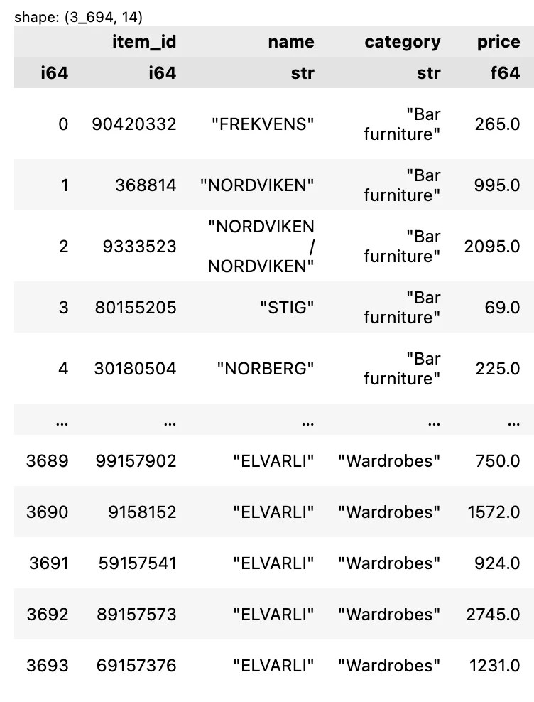
เช่น เรียกใช้ sample_n() เพื่อสุ่มข้อมูลจาก data frame (ตารางข้อมูล):
# Data frame of my friends
friends <- data.frame(
  name = c("Alice", "Bob", "Charlie", "David", "Eve", "Frank", "Grace", "Heidi"),
  age = c(28, 32, 25, 30, 29, 35, 27, 31)
)

# friends data frame:
#       name age
#  1   Alice  28
#  2     Bob  32
#  3 Charlie  25
#  4   David  30
#  5     Eve  29
#  6   Frank  35
#  7   Grace  27
#  8   Heidi  31

# Sample 3 of my friends
sample_n(friends, 3)
ผลลัพธ์:
Error in sample_n(friends, 3) : could not find function "sample_n"
จะเห็นได้ว่า R ส่ง error กลับมา ซึ่งเราแก้ได้โดยติดตั้งและโหลด package ก่อนเรียกใช้งาน sample_n():
💪 ผมขอแนะนำ R Book for Psychologists หนังสือสอนใช้ภาษา R เพื่อการวิเคราะห์ข้อมูลทางจิตวิทยา ที่เขียนมาเพื่อนักจิตวิทยาที่ไม่เคยมีประสบการณ์เขียน code มาก่อน
ในหนังสือ เราจะปูพื้นฐานภาษา R และพาไปดูวิธีวิเคราะห์สถิติที่ใช้บ่อยกัน เช่น:
Correlation
t-tests
ANOVA
Reliability
Factor analysis
🚀 เมื่ออ่านและทำตามตัวอย่างใน R Book for Psychologists ทุกคนจะไม่ต้องพึง SPSS และ Excel ในการทำงานอีกต่อไป และสามารถวิเคราะห์ข้อมูลด้วยตัวเองได้ด้วยความมั่นใจ
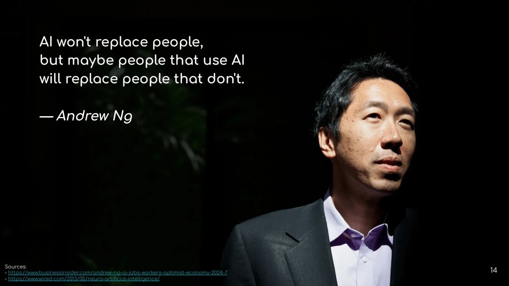
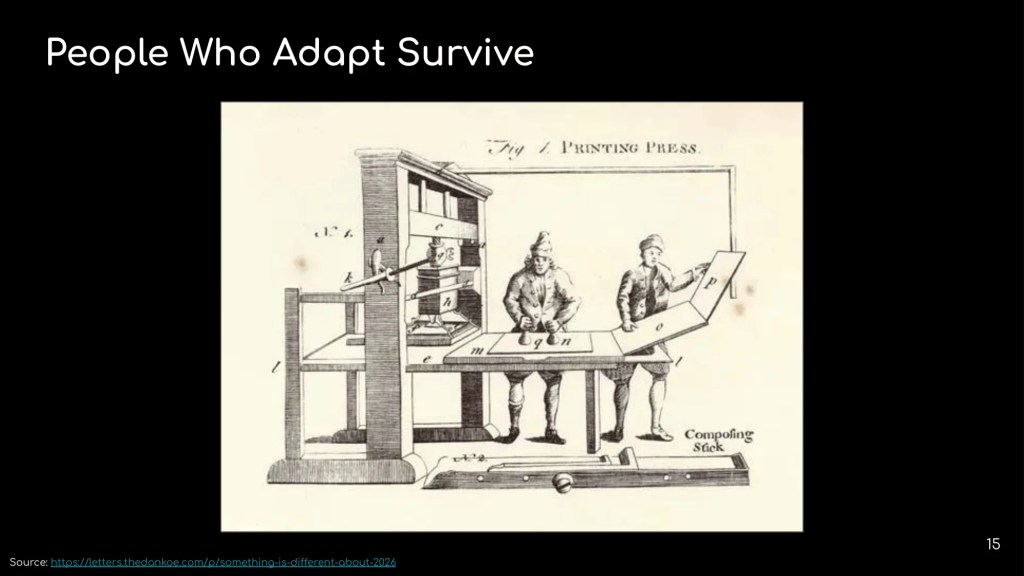
การที่ AI พัฒนาเร็วขึ้นเรื่อย ๆ ทำให้เรามีเวลาปรับตัวน้อยลงเรื่อย ๆ
และตอนนี้ เราเหมือนอยู่ที่ทางแยกที่เราจะต้องเลือกว่า เราจะเรียนรู้การใช้ AI ให้เป็นและอยู่รอดในยุคของ AI หรือเราจะใช้ AI แบบเดิม ๆ และถูกทิ้งไว้ข้างหลัง
The people who will come out of this well won’t be the ones who mastered one tool. They’ll be the ones who got comfortable with the pace of change itself. — Matt Shumer
💼 Part II. Working With AI
.
ข้อ 9. Maslow’s hammer
I suppose it is tempting, if the only tool you have is a hammer, to treat everything as if it were a nail. — Abraham Maslow
Maslow’s hammer เป็น mental model ที่บอกว่า เครื่องมือสามารถจำกัดมุมมองของเราได้
เช่น ถ้าเรามีค้อน เราจะมองทุกอย่างเป็นตะปู
ในยุคของ AI เราอาจมองว่าทุกอย่างแก้ได้ด้วย AI:
ทำงานเร็วขึ้น
ผิดพลาดน้อยลง
มีเวลามากขึ้น
แต่ไม่ใช่ทุกปัญหาจะแก้ได้ด้วย AI เพราะ AI ไม่ใช่เครื่องมือสำหรับแก้ทุกอย่าง
ถ้าเราอยากตอกตะปู เราจะต้องใช้ค้อน ไม่ใช่ AI
การใช้ AI ที่ถูกต้อง คือ เริ่มต้นจากปัญหาและความต้องการของเรา แล้วเลือกเครื่องมือที่ตอบโจทย์ ซึ่งเครื่องมือนั้นอาจจะเป็น AI หรือไม่ก็ได้
.
ข้อ 10. AI is built in man’s image
AI เกิดจากการ train model ด้วยข้อมูลจากอินเทอร์เน็ตซึ่งมาจากมนุษย์
Human -> Data -> Train -> AI
เพราะ AI ถูกสร้างจากข้อมูลของมนุษย์ และเรามองได้ว่า AI เป็นเหมือนเป็นมนุษย์คนหนึ่ง
.
ข้อ 11. AI as capable but junior assistant
ถ้าเรามอง AI เป็นคน AI จะเป็นเหมือนผู้ช่วยที่มีความรู้รอบด้านและมีศักยภาพสูง
แต่สิ่งเดียวที่ผู้ช่วยคนนี้ยังขาดไป คือ ทิศทาง
.
ข้อ 12. Even a fried egg is hard to get right
การทำงานกับ AI ก็เหมือนสั่งไข่ดาว แม้จะดูง่าย แต่ก็ไม่ง่ายอย่างที่คิด
บางครั้ง เราอยากกินไข่ไม่สุก แต่ได้แบบสุกมาแทน
บางครั้ง เราอยากให้ AI สร้างรูปในแบบที่เราคิด แต่ไม่เคยได้ภาพนั้นสักที
ถ้าสิ่งที่ AI ส่งกลับมาไม่ตรงใจ เราควรจะบอก AI ว่าอะไรที่ยังไม่ถูกใจ เพื่อให้ AI ปรับผลลัพธ์และส่งกลับมาให้เราเช็กจนกว่าเราจะพอใจกับงานของ AI
.
ข้อ 16. Be accountable
เราควรจะเช็กงานของ AI ทุกครั้ง เพราะถ้าเราไม่รับผิดชอบกับงานของ AI เราอาจจะเป็นเหมือนทนายความจากออสเตรเลียที่ถูกตรวจสอบ หลังจากศาลพบว่าเอกสารที่ทนายนำส่งเป็นข้อมูลที่ไม่มีอยู่จริง
แม้ทนายจะอ้างว่ารู้เท่าไม่ถึงการณ์ว่า AI ที่บริษัทให้ใช้สามารถสร้างข้อมูลที่ไม่มีอยู่จริงได้ และตัวเองควรตรวจสอบข้อมูลจาก AI ก่อน ศาลยังสั่งให้ทนายงดว่าความด้วยตัวเองเป็นเวลา 2 ปี โดยในระยะเวลานี้จะต้องทำงานเป็นลูกจ้างของคนอื่น และต้องรายงานต่อศาลทุกไตรมาส
ดังนั้น ไม่ว่างานของ AI จะดูดีขนาดไหน เราควรจะตรวจสอบด้วยตัวเองก่อนที่จะนำงานไปใช้จริง
# Set the query
brazil_customers_query = """
SELECT FirstName, LastName, Phone, Email
FROM Customer
WHERE Country = 'Brazil';
"""

# Query the database
df = pd.read_sql(brazil_customers_query, engine)

# Display the df
print(df)
# Set system prompt
system_prompt = """
You are a helpful, cheerful, and optimistic assistant.

Be concise, validate answers, and admit when you don’t know.

Make responses clear, easy to read, and sprinkle in playful emoji.
"""

# Instantiate chat history
chat_history = [
    {
        "role": "system",
        "content": system_prompt
    }
]
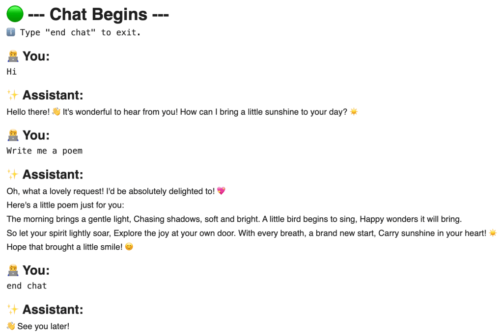
📨 Step 4. Create a Chat Function
ในขั้นที่ 4 เราจะสร้าง function ที่จะทำให้เราถาม-ตอบกับ chatbot แบบ real-time ได้:
# Create a function for chatbot
def chatbot(model="gemini-2.5-flash"):
# Set chat history as global variable
global chat_history
# Print chat header
display(Markdown("# 🟢 --- Chat Begins ---"))
# Print chat instruction
print("ℹ️ Type \\"end chat\\" to exit.")
# Loop through conversation
while True:
# Render user prompt display
display(Markdown("## 🧑💻 You:"))
# Get user input
user_prompt = input("")
# Check if user wants to exit chat
if user_prompt.lower() == "end chat":
# Print goodbye message
display(Markdown("## ✨ Assistant:\\n" + "👋 See you later!"))
# End chat
break
# Append user input to chat history
chat_history.append(
{
"role": "user",
"content": user_prompt
}
)
# Get response
response = client.chat.completions.create(
# Set prompt
messages=chat_history,
# Set model
model=model
)
# Append response to history
chat_history.append(
{
"role": "assistant",
"content": response.choices[0].message.content
}
)
# Render response
display(Markdown("## ✨ Assistant:\\n" + response.choices[0].message.content + "\\n"))
💬 Step 5. Chat
ในขั้นสุดท้าย เราจะเรียกใช้งาน chatbot() เพื่อเริ่มคุยกับ AI เลย:
💪 ผมขอแนะนำ R Book for Psychologists หนังสือสอนใช้ภาษา R เพื่อการวิเคราะห์ข้อมูลทางจิตวิทยา ที่เขียนมาเพื่อนักจิตวิทยาที่ไม่เคยมีประสบการณ์เขียน code มาก่อน
ในหนังสือ เราจะปูพื้นฐานภาษา R และพาไปดูวิธีวิเคราะห์สถิติที่ใช้บ่อยกัน เช่น:
Correlation
t-tests
ANOVA
Reliability
Factor analysis
🚀 เมื่ออ่านและทำตามตัวอย่างใน R Book for Psychologists ทุกคนจะไม่ต้องพึง SPSS และ Excel ในการทำงานอีกต่อไป และสามารถวิเคราะห์ข้อมูลด้วยตัวเองได้ด้วยความมั่นใจ