caret เป็น package ยอดนิยมในภาษา R ในทำ machine learning (ML)
caret ย่อมาจาก Classification And REgression Training และเป็น package ที่ถูกออกแบบมาช่วยให้การทำ ML เป็นเรื่องง่ายโดยมี functions สำหรับทำงานกับ ML workflow เบ็ดเสร็จใน package เดียว
p = สัดส่วนข้อมูลที่เราต้องการแบ่งให้กับ training set
list = ต้องการผลลัพธ์เป็น list (TRUE) หรือ matrix (FALSE)
สำหรับ BostonHousing เราจะแบ่ง 70% เป็น training set และ 30% เป็น test set แบบนี้:
# Set seed for reproducibility
set.seed(888)

# Get train index
train_index <- createDataPartition(BostonHousing$medv, # Specify the outcome
                                   p = 0.7, # Set aside 70% for training set
                                   list = FALSE) # Return as matrix

# Create training set
bt_train <- BostonHousing[train_index, ]

# Create test set
bt_test <- BostonHousing[-train_index, ]
เราสามารถดูจำนวนข้อมลใน training และ test sets ได้ด้วย nrow():
# Check the results
cat("Rows in training set:", nrow(bt_train), "\\n")
cat("Rows in test set:", nrow(bt_test))
ผลลัพธ์:
Rows in training set: 356
Rows in test set: 150
.
🍳 Step 2. Preprocess the Data
ในขั้นที่ 2 เราจะเตรียมข้อมูลเพื่อใช้ในการสร้าง model
# Learn preprocessing on training set
ppc <- preProcess(bt_train[, -14], # Select all predictors
                  method = c("center", "scale"))  # Centre and scale
ตอนนี้ เราจะได้วิธีการเตรียมข้อมูลมาแล้ว ซึ่งเราจะต้องนำไปปรับใช้กับ training และ test sets ด้วย predict() และ cbind() แบบนี้:
Training set:
# Apply preprocessing to training set
bt_train_processed <- predict(ppc,
                              bt_train[, -14])

# Combine the preprocessed training set with outcome
bt_train_processed <- cbind(bt_train_processed,
                            medv = bt_train$medv)
Test set:
# Apply preprocessing to test set
bt_test_processed <- predict(ppc,
                             bt_test[, -14])

# Combine the preprocessed test set with outcome
bt_test_processed <- cbind(bt_test_processed,
                            medv = bt_test$medv)
ตอนนี้ training และ test sets ก็พร้อมที่จะใช้ในการสร้าง model แล้ว
.
👟 Step 3. Train the Model
ในขั้นที่ 3 เราจะสร้าง model กัน
โดยในตัวอย่าง เราจะลองสร้าง k-nearest neighbor (KNN) model ซึ่งทำนายข้อมูลด้วยการดูข้อมูลที่อยู่ใกล้เคียง
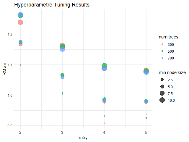
trControl = ค่าที่กำหนดการสร้าง model (ต้องใช้ function ชื่อ trainControl() ในการกำหนด)
tuneGrid = data frame ที่กำหนดค่า hyperparametre เพื่อทำ model tuning และหา model ที่ดีที่สุด
เราสามารถใช้ train() เพื่อสร้าง KNN model ในการทำนายราคาบ้านได้แบบนี้:
# Define training control:
# use k-fold cross-validation where k = 5
trc <- trainControl(method = "cv",
                    number = 5)

# Define grid:
# set k as odd numbers between 3 and 13
grid <- data.frame(k = seq(from = 3,
                           to = 13,
                           by = 2))

# Train the model
knn_model <- train(medv ~ ., # Specify the formula
                   data = bt_train_processed, # Use training set
                   method = "kknn", # Use knn engine
                   trControl = trc, # Specify training control
                   tuneGrid = grid) # Use grid to tune the model
เราสามารถดูรายละเอียดของ model ได้ดังนี้:
# Print the model
knn_model
ผลลัพธ์:
k-Nearest Neighbors

356 samples
 13 predictor

No pre-processing
Resampling: Cross-Validated (5 fold)
Summary of sample sizes: 284, 286, 286, 284, 284
Resampling results across tuning parameters:

  k   RMSE      Rsquared   MAE
   3  4.357333  0.7770080  2.840630
   5  4.438162  0.7760085  2.849984
   7  4.607954  0.7610468  2.941034
   9  4.683062  0.7577702  2.972661
  11  4.771317  0.7508908  3.043617
  13  4.815444  0.7524266  3.053415

RMSE was used to select the optimal model using the smallest value.
The final value used for the model was k = 3.
.
📈 Step 4. Evaluate the Model
ในขั้นสุดท้าย เราจะประเมินความสามารถของ model ในการทำนายราคาบ้านกัน
💪 ผมขอแนะนำ R Book for Psychologists หนังสือสอนใช้ภาษา R เพื่อการวิเคราะห์ข้อมูลทางจิตวิทยา ที่เขียนมาเพื่อนักจิตวิทยาที่ไม่เคยมีประสบการณ์เขียน code มาก่อน
ในหนังสือ เราจะปูพื้นฐานภาษา R และพาไปดูวิธีวิเคราะห์สถิติที่ใช้บ่อยกัน เช่น:
Correlation
t-tests
ANOVA
Reliability
Factor analysis
🚀 เมื่ออ่านและทำตามตัวอย่างใน R Book for Psychologists ทุกคนจะไม่ต้องพึง SPSS และ Excel ในการทำงานอีกต่อไป และสามารถวิเคราะห์ข้อมูลด้วยตัวเองได้ด้วยความมั่นใจ
# A tibble: 6 × 11
  manufacturer model displ  year   cyl trans      drv     cty   hwy fl    class
  <chr>        <chr> <dbl> <int> <int> <chr>      <chr> <int> <int> <chr> <chr>
1 audi         a4      1.8  1999     4 auto(l5)   f        18    29 p     compact
2 audi         a4      1.8  1999     4 manual(m5) f        21    29 p     compact
3 audi         a4      2    2008     4 manual(m6) f        20    31 p     compact
4 audi         a4      2    2008     4 auto(av)   f        21    30 p     compact
5 audi         a4      2.8  1999     6 auto(l5)   f        16    26 p     compact
6 audi         a4      2.8  1999     6 manual(m5) f        18    26 p     compact
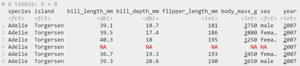
จากผลลัพธ์จะเห็นว่า บาง columns (เช่น manufacturer, model) มีข้อมูลประเภท character ซึ่งเราควระเปลี่ยนเป็น factor เพื่อช่วยให้การสร้าง model มีประสิทธิภาพมากขึ้น:
# Convert character columns to factor

## Get character columns
chr_cols <- c("manufacturer", "model",
              "trans", "drv",
              "fl", "class")

## For-loop through the character columns
for (col in chr_cols) {
  mpg[[col]] <- as.factor(mpg[[col]])
}

## Check the results
str(mpg)
# Split the data

## Set seed for reproducibility
set.seed(123)

## Get training rows
train_rows <- sample(nrow(mpg),
                     nrow(mpg) * 0.7)

## Create a training set
train <- mpg[train_rows, ]

## Create a test set
test <- mpg[-train_rows, ]
💪 ผมขอแนะนำ R Book for Psychologists หนังสือสอนใช้ภาษา R เพื่อการวิเคราะห์ข้อมูลทางจิตวิทยา ที่เขียนมาเพื่อนักจิตวิทยาที่ไม่เคยมีประสบการณ์เขียน code มาก่อน
ในหนังสือ เราจะปูพื้นฐานภาษา R และพาไปดูวิธีวิเคราะห์สถิติที่ใช้บ่อยกัน เช่น:
Correlation
t-tests
ANOVA
Reliability
Factor analysis
🚀 เมื่ออ่านและทำตามตัวอย่างใน R Book for Psychologists ทุกคนจะไม่ต้องพึง SPSS และ Excel ในการทำงานอีกต่อไป และสามารถวิเคราะห์ข้อมูลด้วยตัวเองได้ด้วยความมั่นใจ
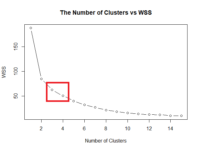
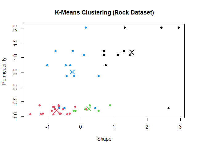
Elbow method หาค่า k ที่ดีที่สุด โดยสร้างกราฟระหว่างค่า k และ within-cluster sum of squares (WSS) หรือระยะห่างระหว่างข้อมูลในกลุ่ม ค่า k ที่ดีที่สุด คือ ค่า k ที่ WSS เริ่มไม่ลดลง
ในภาษา R เราสามารถเริ่มสร้างกราฟได้ โดยเริ่มจากใช้ for loop หา WSS สำหรับช่วงค่า k ที่เราต้องการ
ในตัวอย่าง rock dataset เราจะใช้ช่วงค่า k ระหว่าง 1 ถึง 15:
# Initialise a vector for within cluster sum of squares (wss)
wss <- numeric(15)

# For-loop through the wss
for (k in 1:15) {

  ## Try the k
  km <- kmeans(rock_scaled,
               centers = k,
               nstart = 20)

  ## Get WSS for the k
  wss[k] <- km$tot.withinss
}
จากนั้น ใช้ plot() สร้างกราฟความสัมพันธ์ระหว่างค่า k และ WSS:
# Plot the wss
plot(1:15,
     wss,
     type = "b",
     main = "The Number of Clusters vs WSS",
     xlab = "Number of Clusters",
     ylab = "WSS")
💪 ผมขอแนะนำ R Book for Psychologists หนังสือสอนใช้ภาษา R เพื่อการวิเคราะห์ข้อมูลทางจิตวิทยา ที่เขียนมาเพื่อนักจิตวิทยาที่ไม่เคยมีประสบการณ์เขียน code มาก่อน
ในหนังสือ เราจะปูพื้นฐานภาษา R และพาไปดูวิธีวิเคราะห์สถิติที่ใช้บ่อยกัน เช่น:
Correlation
t-tests
ANOVA
Reliability
Factor analysis
🚀 เมื่ออ่านและทำตามตัวอย่างใน R Book for Psychologists ทุกคนจะไม่ต้องพึง SPSS และ Excel ในการทำงานอีกต่อไป และสามารถวิเคราะห์ข้อมูลด้วยตัวเองได้ด้วยความมั่นใจ
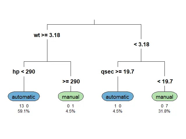
ก่อนนำ mtcars ไปใช้สร้าง classification tree เราจะต้องทำ 2 อย่างก่อน:
อย่างที่ #1. ปรับ column am ให้เป็น factor เพราะสิ่งที่เราต้องการทำนายเป็น categorical data:
# Convert `am` to factor
mtcars$am <- factor(mtcars$am,
                    levels = c(0, 1),
                    labels = c("automatic", "manual"))
# Check the result
class(mtcars$am)
ผลลัพธ์:
[1] "factor"
อย่างที่ #2. Split ข้อมูลเป็น 2 ชุด:
Training set สำหรับสร้าง model
Test set สำหรับประเมิน model
# Set seed for reproducibility
set.seed(500)
# Get training index
train_index <- sample(nrow(mtcars),
                      nrow(mtcars) * 0.7)
# Split the data
train_set <- mtcars[train_index, ]
test_set <- mtcars[-train_index, ]
.
🪴 Train the Model
ตอนนี้ เราพร้อมที่จะสร้าง classification tree ด้วย rpart() แล้ว
สำหรับ classification tree ในบทความนี้ เราจะลองตั้งเงื่อนไขในการปลูกต้นไม้ (control) ดังนี้:
Random forest เป็น tree-based algorithm ที่ช่วยเพิ่มความแม่นยำในการทำนาย โดยสุ่มสร้าง decision trees ต้นเล็กขึ้นมาเป็นกลุ่ม (forest) แทนการปลูก decision tree ต้นเดียว
Decision tree แต่ละต้นใน random forest มีความสามารถในการทำนายแตกต่างกัน ซึ่งบางต้นอาจมีความสามารถที่น้อยมาก
แต่จุดแข็งของ random forest อยู่ที่จำนวน โดย random forest ทำนายผลลัพธ์โดยดูจากผลลัพธ์ในภาพรวม ดังนี้:
Task
Predict by
Regression
ค่าเฉลี่ยของผลลัพธ์การทำนายของทุกต้น
Classification
เสียงส่วนมาก (majority vote)
ดังนั้น แม้ว่า decision tree บางต้นอาจทำนายผิดพลาด แต่โดยรวมแล้ว random forest มีโอกาสที่จะทำนายได้ดีกว่า decision tree ต้นเดียว
ในภาษา R เราสามารถสร้าง random forest ได้ด้วย randomForest() จาก randomForest package ซึ่งต้องการ 3 arguments:
randomFrest(formula, data, ntree)
formula = สูตรในการวิเคราะห์ (ตัวแปรตาม ~ ตัวแปรต้น)
data = dataset ที่ใช้สร้าง model
ntree = จำนวน decision trees ที่ต้องการสร้าง
Note:
เราไม่ต้องกำหนดว่า จะทำ classification หรือ regression model เพราะ randomForest() จะเลือก model ให้อัตโนมัติตามข้อมูลที่เราใส่เข้าไป
💪 ผมขอแนะนำ R Book for Psychologists หนังสือสอนใช้ภาษา R เพื่อการวิเคราะห์ข้อมูลทางจิตวิทยา ที่เขียนมาเพื่อนักจิตวิทยาที่ไม่เคยมีประสบการณ์เขียน code มาก่อน
ในหนังสือ เราจะปูพื้นฐานภาษา R และพาไปดูวิธีวิเคราะห์สถิติที่ใช้บ่อยกัน เช่น:
Correlation
t-tests
ANOVA
Reliability
Factor analysis
🚀 เมื่ออ่านและทำตามตัวอย่างใน R Book for Psychologists ทุกคนจะไม่ต้องพึง SPSS และ Excel ในการทำงานอีกต่อไป และสามารถวิเคราะห์ข้อมูลด้วยตัวเองได้ด้วยความมั่นใจ
  Sepal.Length     Sepal.Width
 Min.   :0.0000   Min.   :0.0000
 1st Qu.:0.2222   1st Qu.:0.3333
 Median :0.4167   Median :0.4167
 Mean   :0.4287   Mean   :0.4406
 3rd Qu.:0.5833   3rd Qu.:0.5417
 Max.   :1.0000   Max.   :1.0000
  Petal.Length     Petal.Width
 Min.   :0.0000   Min.   :0.00000
 1st Qu.:0.1017   1st Qu.:0.08333
 Median :0.5678   Median :0.50000
 Mean   :0.4675   Mean   :0.45806
 3rd Qu.:0.6949   3rd Qu.:0.70833
 Max.   :1.0000   Max.   :1.00000
       Species
 setosa    :50
 versicolor:50
 virginica :50
จะเห็นว่า:
Columns ที่เป็นตัวเลข มีช่วงอยู่ระหว่าง 0 และ 1
เรายังมี column Species อยู่
.
🪓 Split Data
ในการสร้าง KNN model เราควรแบ่ง dataset ที่มีเป็น 2 ส่วน คือ:
Training set: ใช้สำหรับสร้าง model
Test set: ใช้สำหรับประเมิน model
เราเริ่มแบ่งข้อมูลด้วยการสุ่ม row index ที่จะอยู่ใน training set:
# Set seed for reproducibility
set.seed(2025)

# Create a training index
train_index <- sample(1:nrow(iris_normalised),
                      0.7 * nrow(iris_normalised))
จากนั้น subset ข้อมูลด้วย row index ที่สุ่มไว้:
# Split the data
train_set <- iris_normalised[train_index, ]
test_set <- iris_normalised[-train_index, ]
.
🏷️ Separate Features From Label
ขั้นตอนสุดท้ายในการเตรียมข้อมูล คือ แยก features หรือ X (columns ที่จะใช้ทำนาย) ออกจาก label หรือ Y (สิ่งที่ต้องการทำนาย):
# Separate features from label

## Training set
train_X <- train_set[, 1:4]
train_Y <- train_set$Species

## Test set
test_X <- test_set[, 1:4]
test_Y <- test_set$Species
4️⃣ Step 4. Train a KNN Model
ขั้นที่สี่เป็นขั้นที่เราสร้าง KNN model ขึ้นมา โดยเรียกใช้ knn() จาก class package
ทั้งนี้ knn() ต้องการ input 3 อย่าง:
train: fatures จาก training set
test: feature จาก test set
cl: label จาก training set
k: จำนวนข้อมูลใกล้เคียงที่จะใช้ทำนายผลลัพธ์
# Train a KNN model
pred <- knn(train = train_X,
            test = test_X,
            cl = train_Y,
            k = 5)
ในตัวอย่าง เรากำหนด k = 5 เพื่อทำนายผลลัพธ์โดยดูจากข้อมูลที่ใกล้เคียง 5 อันดับแรก
5️⃣ Step 5. Evaluate the Model
หลังจากได้ model แล้ว เราประเมินประสิทธิภาพของ model ในการทำนายผลลัพธ์ ซึ่งเราทำได้ง่าย ๆ โดยคำนวณ accuracy หรือสัดส่วนของข้อมูลที่ model ตอบถูกต่อจำนวนข้อมูลทั้งหมด:
Accuracy = Correct predictions / Total predictions
จากผลลัพธ์ เราจะเห็นว่า model มีความแม่นยำสูงถึง 96%
🍩 Bonus: Fine-Tuning
ในบางครั้ง ค่า k ที่เราตั้งไว้ อาจไม่ได้ทำให้เราได้ KNN model ที่ดีที่สุด
แทนที่เราจะแทนค่า k ใหม่ไปเรื่อย ๆ เราสามารถใช้ for loop เพื่อหาค่า k ที่ทำให้เราได้ model ที่ดีที่สุดได้
ให้เราเริ่มจากสร้าง vector ที่มีค่า k ที่ต้องการ:
# Create a set of k values
k_values <- 1:20
และ vector สำหรับเก็บค่า accuracy ของค่า k แต่ละตัว:
# Createa a vector for accuracy results
accuracy_results <- numeric(length(k_values))
แล้วใช้ for loop เพื่อหาค่า accuracy ของค่า k:
# For-loop through the k values
for (i in seq_along(k_values)) {

  ## Set the k value
  k <- k_values[i]

  ## Create a KNN model
  predictions <- knn(train = train_X,
                     test = test_X,
                     cl = train_Y,
                     k = k)

  ## Create a confusion matrix
  cm <- table(Predicted = predictions,
              Actual = test_Y)

  ## Calculate accuracy
  accuracy_results[i] <- sum(diag(cm)) / sum(cm)
}

# Find the best k and the corresponding accuracy
best_k <- k_values[which.max(accuracy_results)]
best_accuracy <- max(accuracy_results)

# Print best k and accuracy
cat(paste("Best k:", best_k),
    paste("Accuracy:", round(best_accuracy, 2)),
    sep = "\n")
ผลลัพธ์:
Best k: 12
Accuracy: 0.98
แสดงว่า ค่า k ที่ดีที่สุด คือ 12 โดยมี accuracy เท่ากับ 98%
นอกจากนี้ เรายังสามารถสร้างกราฟ เพื่อช่วยทำความเข้าใจผลของค่า k ต่อ accuracy:
# Plot the results
plot(k_values,
     accuracy_results,
     type = "b",
     pch = 19,
     col = "blue",
     xlab = "Number of Neighbors (k)",
     ylab = "Accuracy",
     main = "KNN Model Accuracy for Different k Values")
grid()
ผลลัพธ์:
จะเห็นได้ว่า k = 12 ให้ accuracy ที่ดีที่สุด และ k = 20 ให้ accuracy ต่ำที่สุด ส่วนค่า k อื่น ๆ ให้ accuracy ในช่วง 93 ถึง 96%
💪 ผมขอแนะนำ R Book for Psychologists หนังสือสอนใช้ภาษา R เพื่อการวิเคราะห์ข้อมูลทางจิตวิทยา ที่เขียนมาเพื่อนักจิตวิทยาที่ไม่เคยมีประสบการณ์เขียน code มาก่อน
ในหนังสือ เราจะปูพื้นฐานภาษา R และพาไปดูวิธีวิเคราะห์สถิติที่ใช้บ่อยกัน เช่น:
Correlation
t-tests
ANOVA
Reliability
Factor analysis
🚀 เมื่ออ่านและทำตามตัวอย่างใน R Book for Psychologists ทุกคนจะไม่ต้องพึง SPSS และ Excel ในการทำงานอีกต่อไป และสามารถวิเคราะห์ข้อมูลด้วยตัวเองได้ด้วยความมั่นใจ
  model            mpg
  <chr>          <dbl>
1 Toyota Corolla  33.9
2 Fiat 128        32.4
3 Honda Civic     30.4
4 Lotus Europa    30.4
5 Fiat X1-9       27.3
6 Porsche 914-2   26
# ℹ 4 more rows
# ℹ Use `print(n = ...)` to see more rows
💪 ผมขอแนะนำ R Book for Psychologists หนังสือสอนใช้ภาษา R เพื่อการวิเคราะห์ข้อมูลทางจิตวิทยา ที่เขียนมาเพื่อนักจิตวิทยาที่ไม่เคยมีประสบการณ์เขียน code มาก่อน
ในหนังสือ เราจะปูพื้นฐานภาษา R และพาไปดูวิธีวิเคราะห์สถิติที่ใช้บ่อยกัน เช่น:
Correlation
t-tests
ANOVA
Reliability
Factor analysis
🚀 เมื่ออ่านและทำตามตัวอย่างใน R Book for Psychologists ทุกคนจะไม่ต้องพึง SPSS และ Excel ในการทำงานอีกต่อไป และสามารถวิเคราะห์ข้อมูลด้วยตัวเองได้ด้วยความมั่นใจ
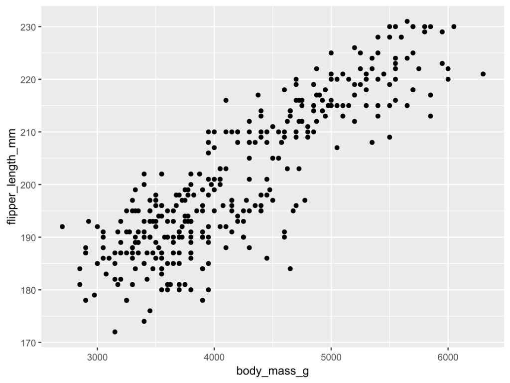
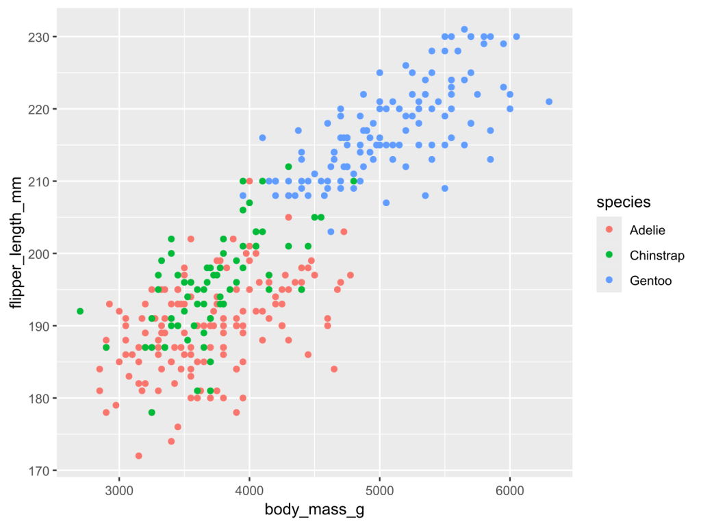
ggplot2 เป็น package สำหรับ data visualisation ในภาษา R และเป็นเครื่องมือสร้างกราฟที่มืออาชีพนิยม ตั้งแต่นักวิจัยในการตีพิมพ์ผลงาน ไปจนถึงสำนักข่าวระดับโลกอย่าง BBC และ Financial Times
💪 ผมขอแนะนำ R Book for Psychologists หนังสือสอนใช้ภาษา R เพื่อการวิเคราะห์ข้อมูลทางจิตวิทยา ที่เขียนมาเพื่อนักจิตวิทยาที่ไม่เคยมีประสบการณ์เขียน code มาก่อน
ในหนังสือ เราจะปูพื้นฐานภาษา R และพาไปดูวิธีวิเคราะห์สถิติที่ใช้บ่อยกัน เช่น:
Correlation
t-tests
ANOVA
Reliability
Factor analysis
🚀 เมื่ออ่านและทำตามตัวอย่างใน R Book for Psychologists ทุกคนจะไม่ต้องพึง SPSS และ Excel ในการทำงานอีกต่อไป และสามารถวิเคราะห์ข้อมูลด้วยตัวเองได้ด้วยความมั่นใจ
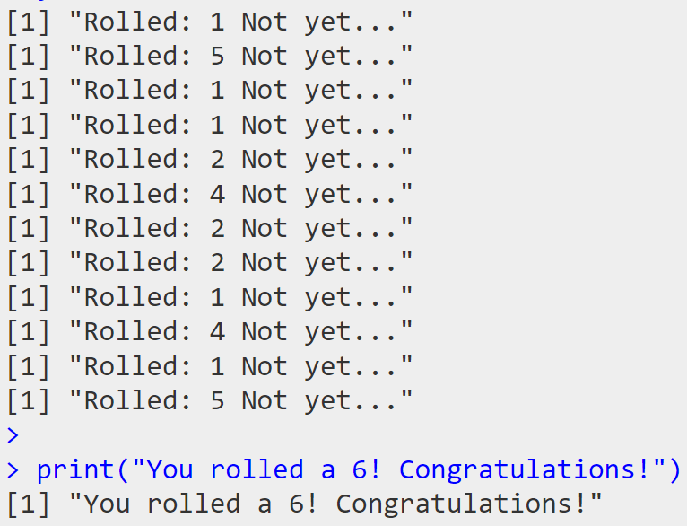
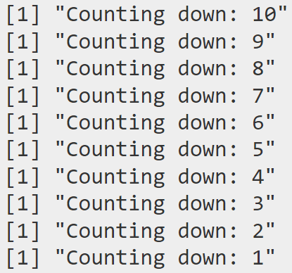
time <- 10 # Start countdown
while (time > 0) {
print(paste("Counting down:", time))
time <- time - 1
}
ถ้าเราไม่ใส่ break, while loop ของเราจะนับเลขถึง 0:
while without break
.
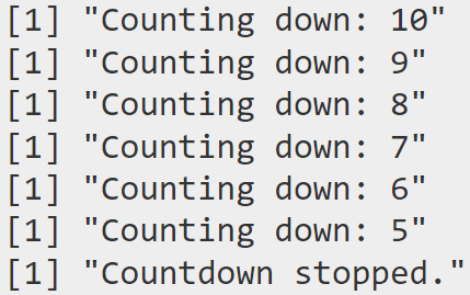
แต่ถ้าเราใส่ break เข้าไป while loop จะหยุดนับ ณ ตัวเลขที่เรากำหนด:
time <- 10 # Start countdown
while (time > 0) {
if (time == 4) {
print("Countdown stopped.")
break # Stop the loop when time reaches 4
}
print(paste("Counting down:", time))
time <- time - 1
}
ผลลัพธ์:
while with break
จะเห็นได้ว่า break ทำให้ while loop หยุดทำงาน เมื่อนับถึง 4
💪 Summary
ในบทความนี้ เราเรียนรู้วิธีเขียน control flow ใน R กัน:
💪 ผมขอแนะนำ R Book for Psychologists หนังสือสอนใช้ภาษา R เพื่อการวิเคราะห์ข้อมูลทางจิตวิทยา ที่เขียนมาเพื่อนักจิตวิทยาที่ไม่เคยมีประสบการณ์เขียน code มาก่อน
ในหนังสือ เราจะปูพื้นฐานภาษา R และพาไปดูวิธีวิเคราะห์สถิติที่ใช้บ่อยกัน เช่น:
Correlation
t-tests
ANOVA
Reliability
Factor analysis
🚀 เมื่ออ่านและทำตามตัวอย่างใน R Book for Psychologists ทุกคนจะไม่ต้องพึง SPSS และ Excel ในการทำงานอีกต่อไป และสามารถวิเคราะห์ข้อมูลด้วยตัวเองได้ด้วยความมั่นใจ