polars เป็น package สำหรับทำงานกับข้อมูลในรูปแบบตาราง (tabular data) ใน Python และถูกพัฒนาด้วย Rust และ Apache Arrow ซึ่งทำให้ polars ประมวลผลได้เร็วและมีประสิทธิภาพสูง
polars เป็นทางเลือกสำหรับคนที่เบื่อกับข้อจำกัดของ pandas ซึ่งเป็น package ยอดนิยมสำหรับทำงานกับข้อมูลในรูปแบบตาราง โดย polars ได้เปรียบ pandas อยู่ 3 อย่าง:
- Fast: ประมวลผลเร็วกว่า
- Intuitive: มี syntax ที่ใช้ง่ายกว่า
- Lazy: รองรับการเขียนแบบ lazy evaluation (ดูรายละเอียดเพิ่มเติมด้านล่าง) ทำให้ประมวลผลได้มีประสิทธิภาพมากกว่า
Note: ดูวิธีการใช้ pandas ได้ที่บทความนี้
ในบทความนี้ เราจะมาดูวิธีใช้ polars ผ่านตัวอย่างการทำงานกับ IKEA Products dataset ที่มีข้อมูลเฟอร์นิเจอร์จาก IKEA กัน
โดยบทความแบ่งเป็น 9 ส่วนดังนี้:
- Import package and dataset: โหลด package และ dataset
- Explore: สำรวจ dataset ก่อนทำงานกับข้อมูล
- Select: เลือกข้อมูล
- Filter: กรองข้อมูล
- Sort: จัดเรียงข้อมูล
- Aggregate: หาค่าทางสถิติ
- Mutate: เพิ่ม ลบ แก้ไข column
- Lazy: การทำงานแบบ lazy
- Chaining: การเชื่อมต่อ function
ถ้าพร้อมแล้ว ไปเริ่มกันเลย
- 📦 Section 1. Import Package & Dataset
- 🧭 Section 2. Explore
- 🫳 Section 3. Select
- 👀 Section 4. Filter
- ↕️ Section 5. Sort
- 🧮 Section 6. Aggregate
- 💪 Section 7. Mutate
- 🥱 Section 8. Lazy
- 🔗 Section 9. Chaining
- ⭐️ Summary
- ⏭️ Next Step: DIY
- 📃 References
📦 Section 1. Import Package & Dataset
ในขั้นแรก เราจะโหลด package และ dataset ที่จะใช้งานกันก่อน
เราจะโหลด package ด้วย import แบบนี้:
import polars as pl
Note: ก่อนโหลด เราจะต้องติดตั้ง package ซึ่งเราสามารถทำได้ด้วย pip install
และโหลด dataset ด้วย read_csv() เพราะข้อมูลเป็นไฟล์ CSV:
df = pl.read_csv("ikea_products.csv")
ตอนนี้ เรามีข้อมูลพร้อมจะทำงานต่อแล้ว
🧭 Section 2. Explore
ในขั้นที่ 2 เราจะสำรวจข้อมูลที่เพิ่งโหลดเสร็จ ซึ่งเราทำได้ 5 วิธี:
shapeschemahead()glimpse()describe()
.
🔷 2.1 shape
shape เป็น attribute สำหรับเช็กจำนวน rows และ columns ใน dataset:
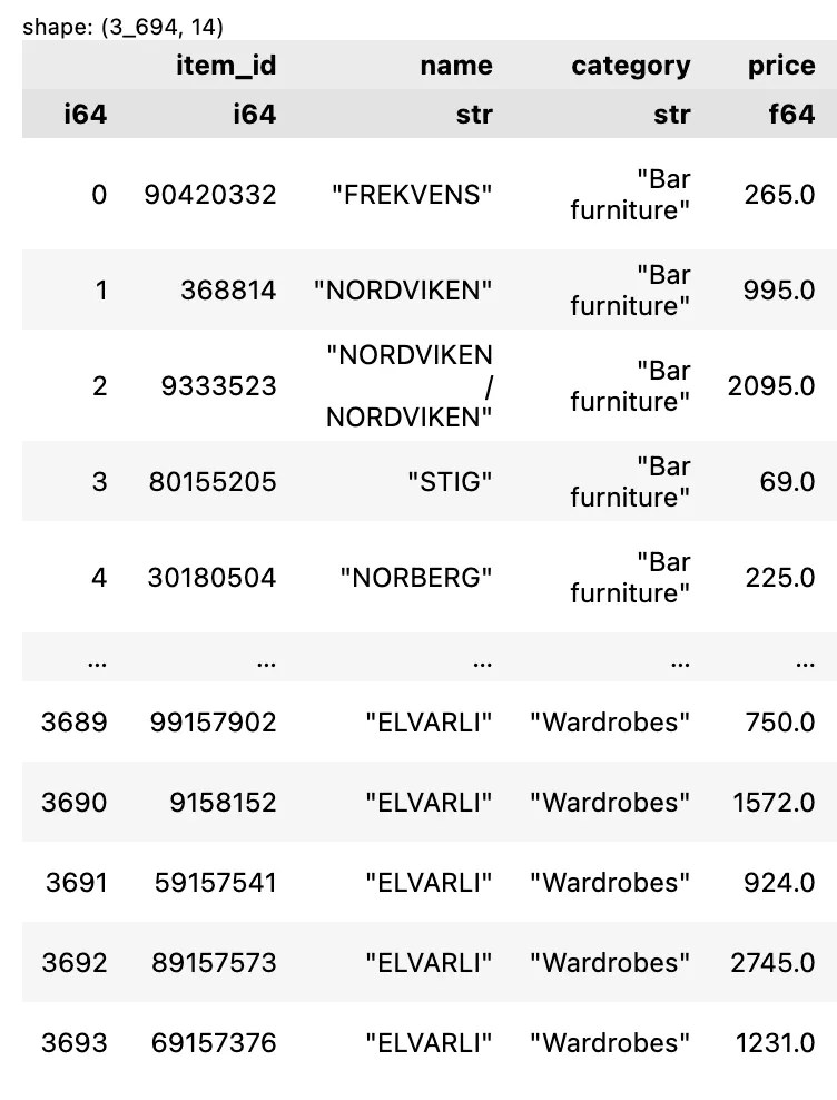
df.shape
ผลลัพธ์:
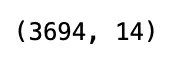
จากผลลัพธ์ จะเห็นว่า dataset มีข้อมูล 3,694 rows และมี 14 columns
.
🗺️ 2.2 schema
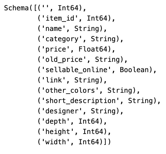
schema เป็น attribute สำหรับแสดงชื่อและประเภทข้อมูลของ columns:
df.schema
ผลลัพธ์:
.
🐵 2.3 head()
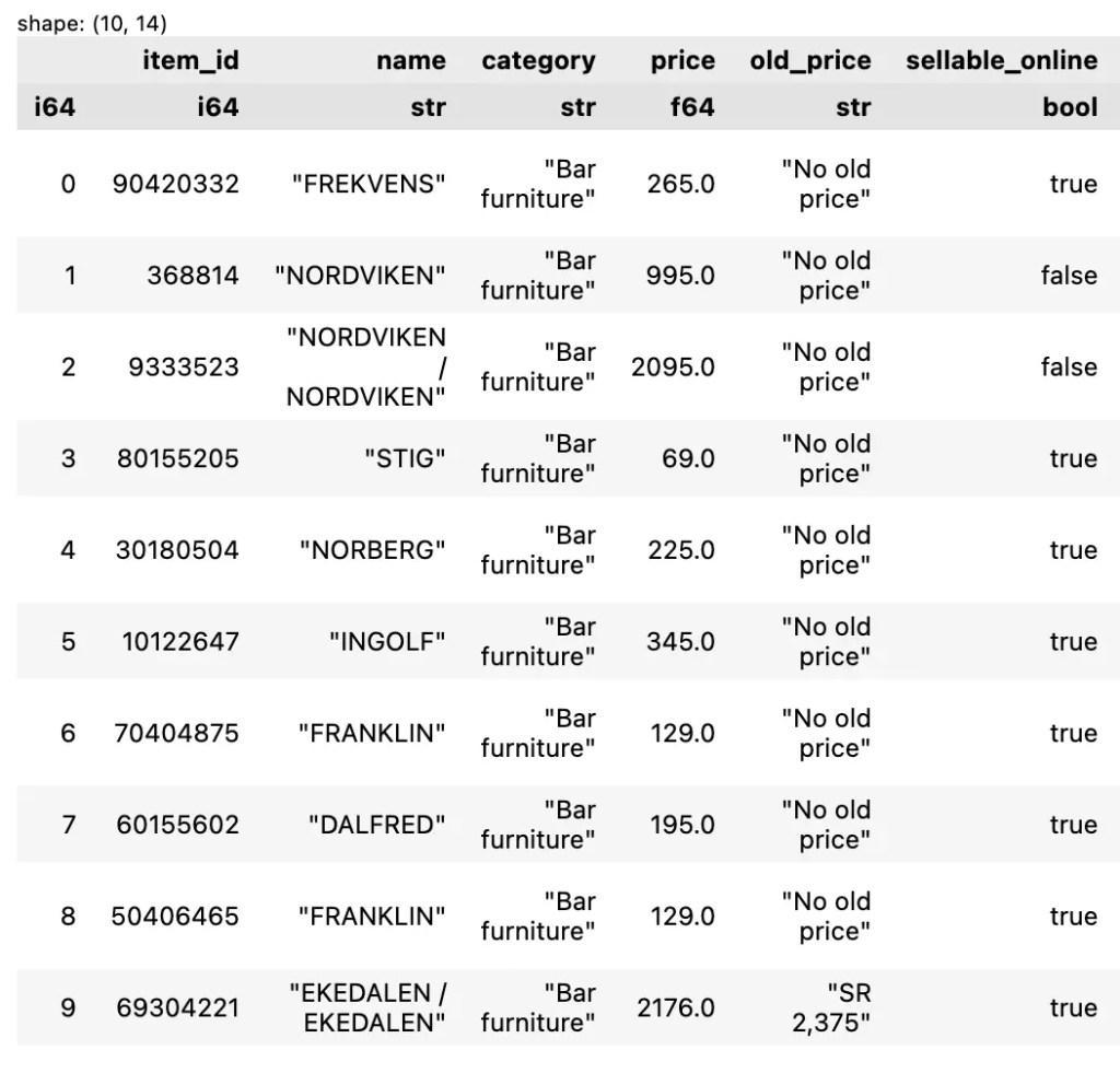
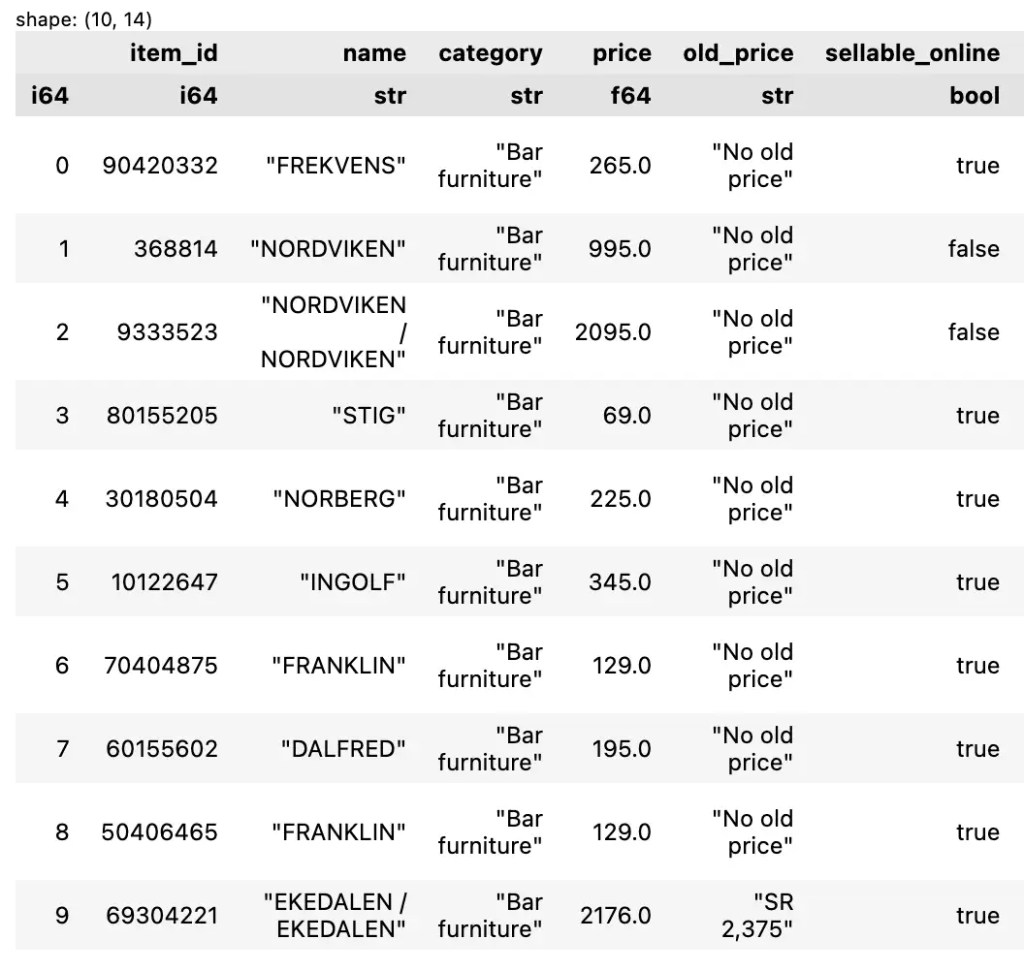
head() เป็น method สำหรับดู n rows แรกของข้อมูล เช่น ดู 10 แรกของข้อมูล:
df.head(10)
ตัวอย่างผลลัพธ์:
.
🔎 2.4 glimpse()
glimpse() เป็น method สำหรับดูโครงสร้างข้อมูล ซึ่งประกอบด้วย:
- จำนวน rows และ columns
- ชื่อ column
- ประเภทข้อมูล
- ตัวอย่างข้อมูล
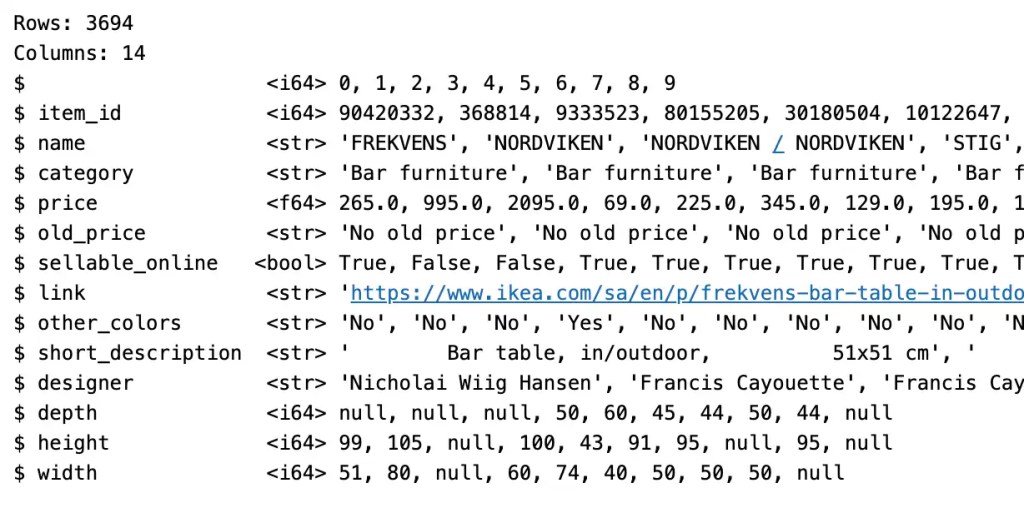
df.glimpse()
ตัวอย่างผลลัพธ์:
.
.
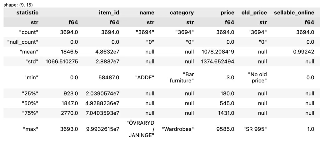
📝 2.5 describe()
describe() เป็น method สำหรับแสดง summary statistics ของ columns:
count: จำนวนข้อมูลnull_count: จำนวนข้อมูลที่เป็นค่าว่างmean: ค่าเฉลี่ยstd: ค่าเบี่ยงเบนมาตรฐาน (standard deviation)min: ค่าต่ำสุด25%,50%,75%: ข้อมูลที่ quartile ที่ 1, 2, และ 3max: ค่าสูงสุด
df.describe()
ตัวอย่างผลลัพธ์:
🫳 Section 3. Select
เรามี 2 วิธีในการเลือก rows และ columns จากข้อมูล:
- ใช้
[] - ใช้
slice()และselect()
.
🔲 3.1 Using []
เราจะใช้ [] โดยกำหนด rows และ columns ที่ต้องการแบบนี้:
df[rows, cols]
ถ้าเราต้องการ rows หรือ columns ทั้งหมด ให้เราเว้นข้อมูลส่วนนั้นไว้ เช่น เลือกข้อมูล 10 rows แรก และ columns ทั้งหมด:
df[:10]
ตัวอย่างผลลัพธ์:

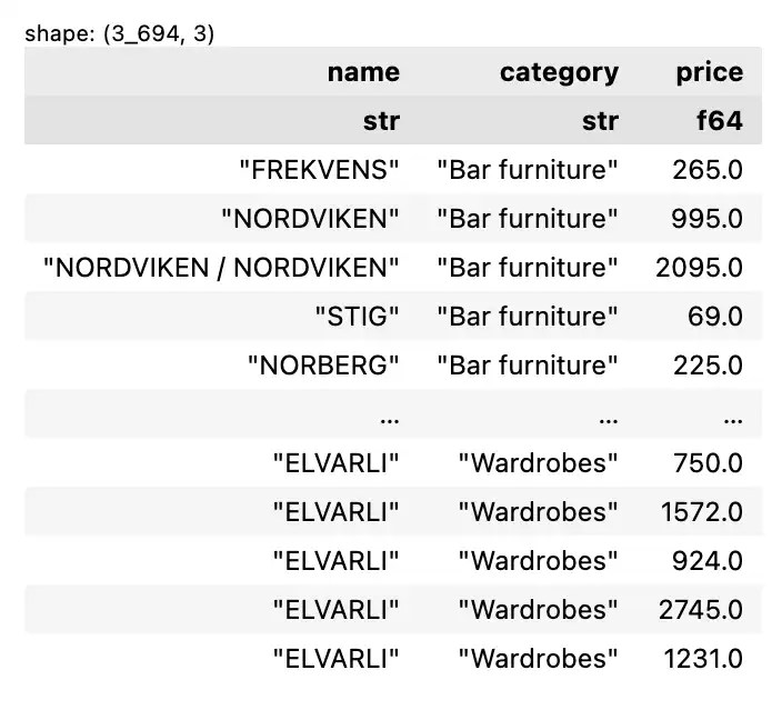
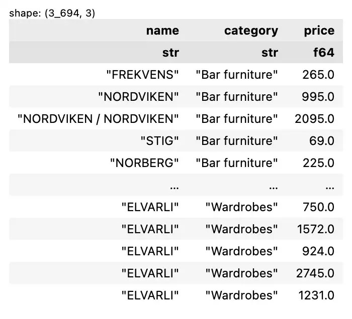
หรือเลือกเฉพาะ columns ชื่อ ประเภท และราคา และ rows ทั้งหมด:
df[["name", "category", "price"]]
ผลลัพธ์:
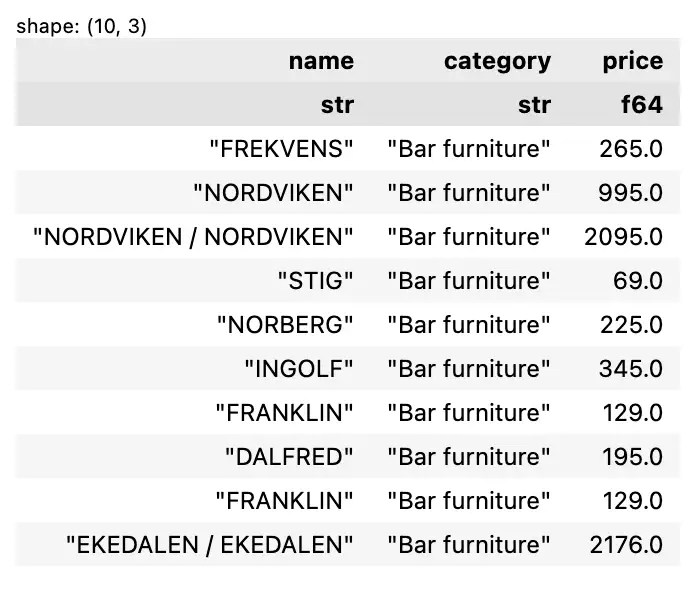
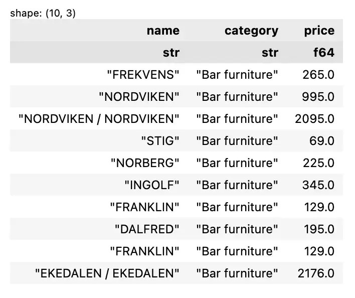
ถ้าต้องการทั้ง rows และ columns ให้เรากำหนดทั้งสองอย่าง เช่น ข้อมูล 10 rows แรก โดยเลือกเฉพาะ columns ชื่อ ประเภท และราคา:
df[0:10, ["name", "category", "price"]]
ผลลัพธ์:
.
🔪 3.2 Using slice() & select()
เราสามารถใช้ slice() และ select() เพื่อเลือกข้อมูลแทนการใช้ [] ได้ โดย:
- ใช้
slice()เลือก rows - ใช้
select()เลือก columns
เช่น เลือกข้อมูล 10 rows แรก:
df.slice(0, 10)
ตัวอย่างผลลัพธ์:
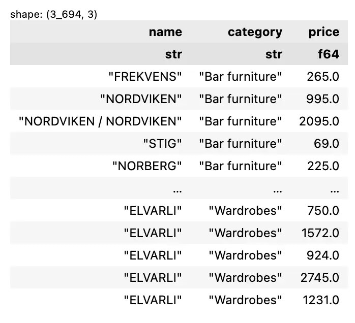
เลือก columns ชื่อ ประเภท และราคา:
df.select(["name", "category", "price"])
ผลลัพธ์:
สุดท้าย เราสามารถใช้ทั้ง slice() และ select() ร่วมกันเพื่อเลือกทั้ง rows และ columns ได้แบบนี้:
df.slice(0, 10).select(["name", "category", "price"])
ผลลัพธ์:
👀 Section 4. Filter
เรากรองข้อมูลได้ด้วย filter() ซึ่งรับรองการกรองแบบ 1 เงื่อนไข และมากกว่า 1 เงื่อนไข
.
☝️ 4.1 One Condition
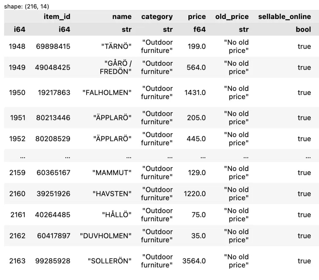
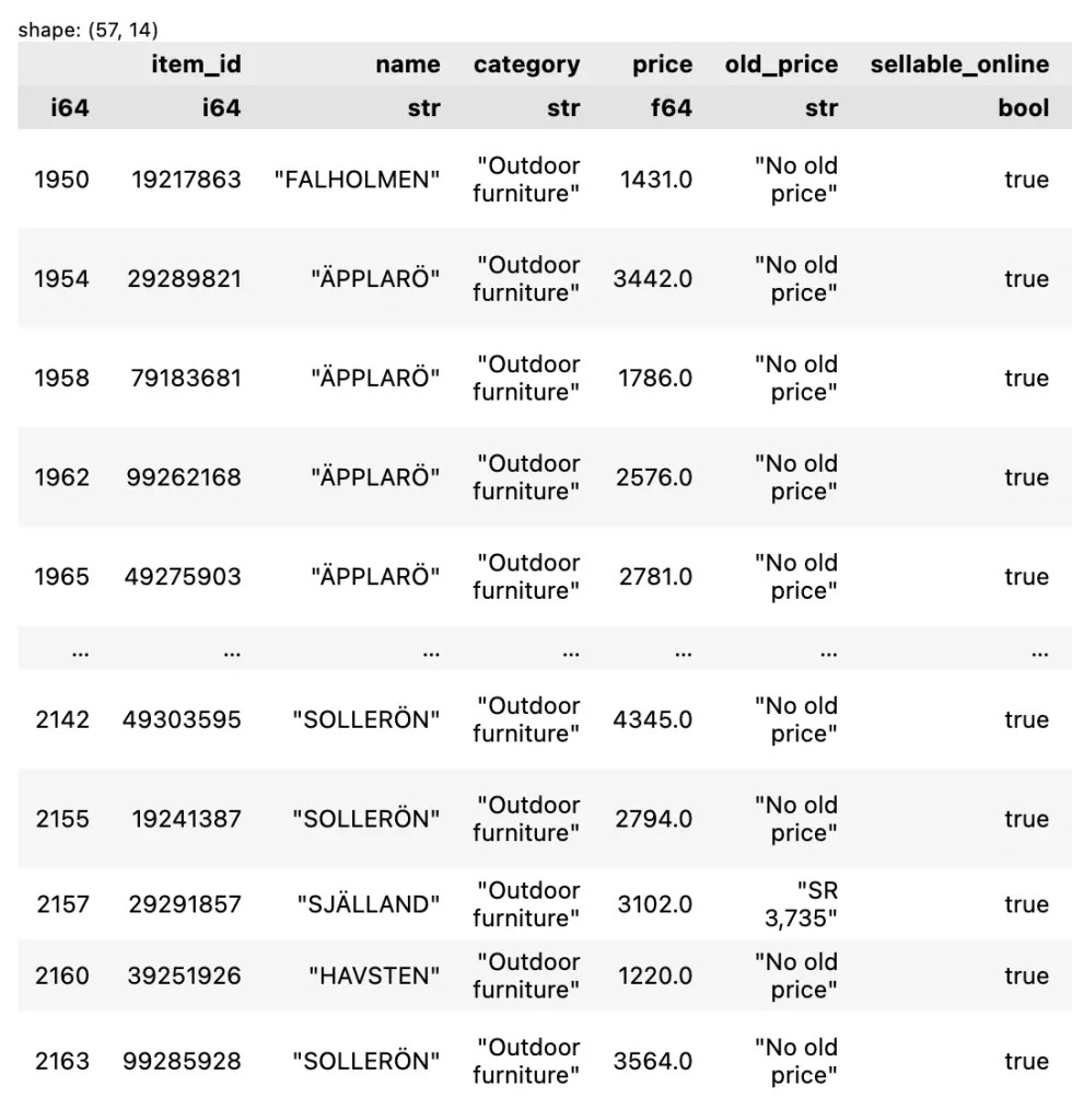
ตัวอย่างการกรองแบบ 1 เงื่อนไข เช่น เลือกเฉพาะข้อมูลของ outdoor furniture:
df.filter(pl.col("category") == "Outdoor furniture")
Note: สังเกตว่า เราใช้ col() เพื่อระบุ column ที่ต้องการ
ตัวอย่างผลลัพธ์:
.
🖐️ 4.2 Multiple Conditions
สำหรับการกรองหลายเงื่อนไข เราจะใช้ logical operator ช่วย:
| Operator | Meaning |
|---|---|
& | And |
| | | Or |
~ | Not |
เช่น เลือกข้อมูล outdoor furniture ที่ราคาสูงกว่า 1,000:
df.filter(
    (pl.col("category") == "Outdoor furniture") &
    (pl.col("price") > 1000)
)
ตัวอย่างผลลัพธ์:
↕️ Section 5. Sort
สำหรับจัดลำดับข้อมูล เราจะใช้ sort() ซึ่งรองรับการใช้งาน 3 กรณี:
- Ascending: เรียงจากน้อยไปมาก (A–Z)
- Descending: เรียงจากมากไปน้อย (Z–A)
- Multiple columns: เรียงลำดับหลาย columns พร้อมกัน
.
⬆️ 5.1 Ascending
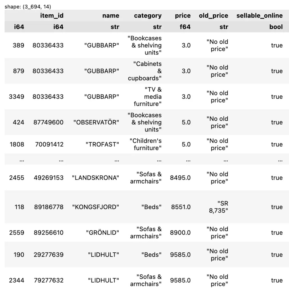
Default ในการจัดลำดับของ sort() คือ เรียงจากน้อยไปมาก เช่น จัดเรียงข้อมูลตามราคา:
df.sort("price")
ตัวอย่างผลลัพธ์:
.
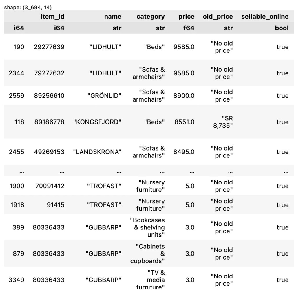
⬇️ 5.2 Descending
ถ้าต้องการจัดเรียงแบบมากไปน้อย เราจะต้องกำหนด argument descending=True:
df.sort("price", descending=True)
ตัวอย่างผลลัพธ์:
.
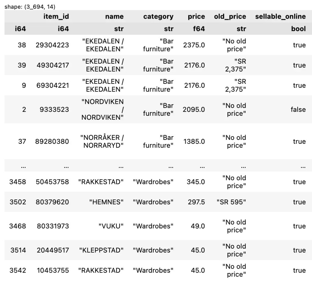
🖐️ 5.3 Multiple Columns
ถ้าต้องการจัดลำดับหลาย columns พร้อมกัน เราจะกำหนด columns และวิธีจัดเรียง (ascending vs descending) เช่น จัดเรียงตามประเภทเฟอร์นิเจอร์ (A–Z) และราคา (Z–A):
df.sort(
    ["category", "price"],
    descending=[False, True]
)
ตัวอย่างผลลัพธ์:
🧮 Section 6. Aggregate
Aggregate คือ การสรุปข้อมูล เช่น หาค่าเฉลี่ย และทำได้ 2 วิธี:
- แบบไม่จัดกลุ่ม ด้วยคำสั่ง
select() - แบบจัดกลุ่ม ด้วยคำสั่ง
group_by()และagg()
.
🏠 6.1 Basic
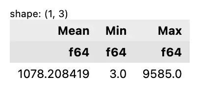
ตัวอย่างสรุปข้อมูลโดยไม่จัดกลุ่ม เช่น หาค่าเฉลี่ย ค่าต่ำสุด และค่าสูงสุดของราคาเฟอร์นิเจอร์:
df.select(
    pl.col("price").mean().alias("Mean"),
    pl.col("price").min().alias("Min"),
    pl.col("price").max().alias("Max")
)
Note: alias() ใช้ตั้งชื่อ column
ผลลัพธ์:
.
🏘️ 6.2 Group By
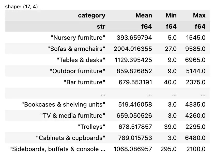
ตัวอย่างสรุปข้อมูลแบบจัดกลุ่ม เช่น หาค่าเฉลี่ย ค่าต่ำสุด และค่าสูงสุดของราคาเฟอร์นิเจอร์ ตามประเภทเฟอร์นิเจอร์:
df.group_by("category").agg(
    pl.col("price").mean().alias("Mean"),
    pl.col("price").min().alias("Min"),
    pl.col("price").max().alias("Max")
)
ตัวอย่างผลลัพธ์:
💪 Section 7. Mutate
Mutate หมายถึง การปรับเปลี่ยน columns ที่มีอยู่ เช่น เพิ่มหรือลบ columns
.
➕ 7.1 Add Columns
ตัวอย่างการเพิ่ม columns เช่น:
- เพิ่ม column ส่วนลด (
discount) โดยราคามากกว่า 1,000 จะลด 15% และราคาน้อยกว่านั้นจะลด 10% และ - เพิ่ม column แสดงราคาหลังใช้ส่วนลดแล้ว (
price_discounted)
เราสามารถเขียน code ได้ดังนี้:
df.with_columns(
    discount = pl.when(pl.col("price") > 1000)
    .then(0.15)
    .otherwise(0.10),
).with_columns(
    price_discounted = pl.col("price") * (1 - pl.col("discount"))
)
Note: เราใช้ when(), then(), otherwise() ช่วยกำหนดเงื่อนไขที่ต้องการ
ตัวอย่างผลลัพธ์:
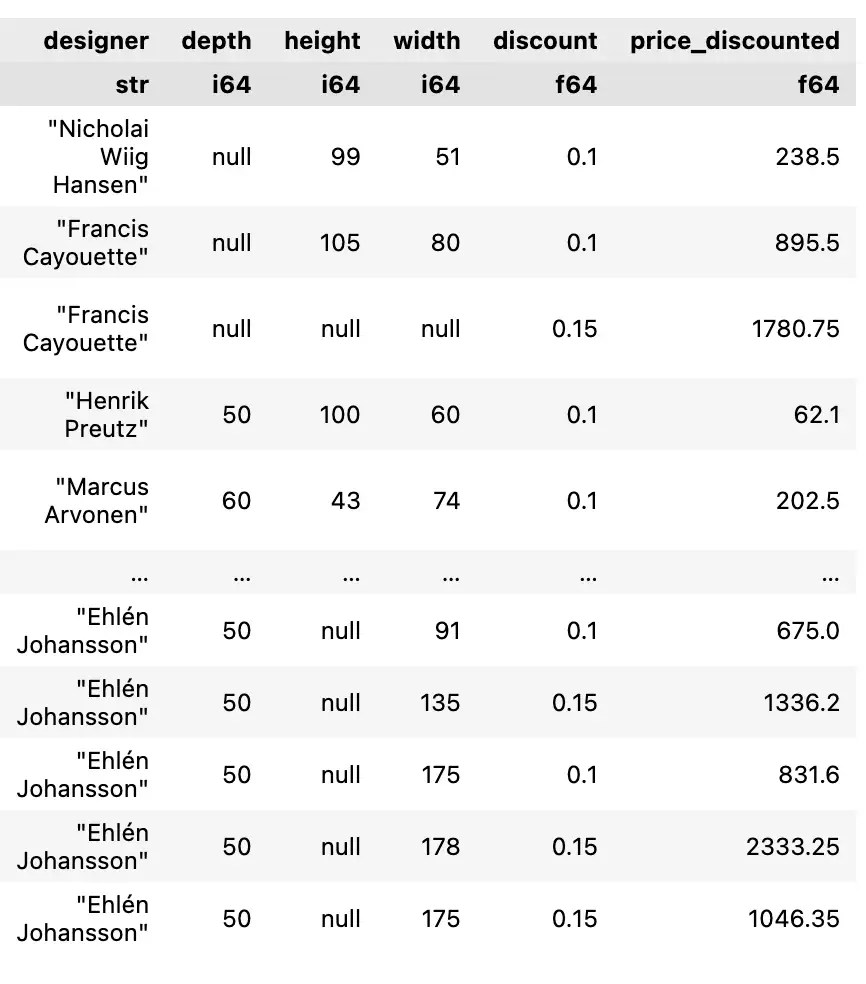
สังเกตว่า columns ใหม่จะอยู่ต่อท้ายสุด
.
🗑️ 7.2 Remove Columns
เราลบ column ได้ด้วย drop() เช่น ลบ columns ราคาเก่า (old_price) และการขายออนไลน์ (sellable_online):
df.drop(["old_price", "sellable_online"])
ตัวอย่างผลลัพธ์:
🥱 Section 8. Lazy
Lazy evaluation เป็นการประมวลผลที่จะรันก็ต่อเมื่อได้รับคำสั่ง ซึ่งช่วยให้การทำงานมีประสิทธิภาพมากขึ้น เพราะการประมวลผลจะไม่เกิดขึ้นจนกว่าจะจำเป็น
Note: การประมวลผลในทันทีโดยไม่รอคำสั่ง เรียกว่า eager evaluation
การทำงานแบบ lazy evaluation มีอยู่ 3 ขั้นตอน:
ขั้นที่ 1. สร้าง LazyFrame ซึ่งเป็นข้อมูลสำหรับ lazy evaluation ด้วย lazy():
df_lz = df.lazy()
ขั้นที่ 2. เขียนคำสั่งที่ต้องการ เช่น เลือก columns:
execution = df_lz.select(["name", "category", "price"])
ขั้นที่ 3. สั่งให้ประมวลผลด้วยคำสั่ง collect():
execution.collect()
ผลลัพธ์:
🔗 Section 9. Chaining
Chaining เป็นการเชื่อมต่อ function เพื่อส่งผลลัพธ์จาก function หนึ่งไปยังอีก function หนึ่ง:
df.function1().function2().function3()...
Chaining ช่วยให้เราตอบโจทย์ที่ซับซ้อนขึ้นได้ เช่น:
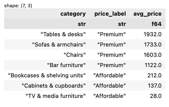
สำหรับเฟอร์นิเจอร์ที่ Francis Cayouette ออกแบบ ประเภทไหนจัดว่าเป็น “Premium” (ราคาสูงกว่า 1,000) และ “Affordable” (ราคาน้อยกว่า 1,000)
เราสามารถใช้ polars เพื่อตอบโจทย์ได้แบบนี้:
df_lz.filter(
    pl.col("designer") == "Francis Cayouette"
).group_by(
    "category"
).agg(
    pl.col("price").mean().round().alias("avg_price")
).with_columns(
    pl.when(pl.col("avg_price") > 1000)
    .then(pl.lit("Premium"))
    .otherwise(pl.lit("Affordable"))
    .alias("price_label")
).sort(
    "avg_price",
    descending=True
).select(
    [
        "category",
        "price_label",
        "avg_price"
    ]
).collect()
ผลลัพธ์:
⭐️ Summary
ในบทความนี้ เราได้เห็นวิธีการใช้ polars เพื่อทำงานกับข้อมูลในรูปแบบตาราง ซึ่งสามารถสรุปเป็นการเขียน code 9 กลุ่มได้ดังนี้:
Section 1. Import package & dataset:
import polars as plpl.read_csv()
Section 2. Explore:
df.shapedf.schemadf.head()df.glimpse()df.describe()
Section 3. Select:
df[rows, cols]pl.slice()pl.select()
Section 4. Filter:
df.filter()pl.col()&,|,~
Section 5. Sort:
df.sort()
Section 6. Aggregate:
df.select()df.group_by().agg()alias()
Section 7. Mutate:
df.with_columns()pl.when().then().otherwise()df.drop()
Section 8. Lazy:
df.lazy()collect()
Section 9. Chaining:
df.function1().function2().function()...
⏭️ Next Step: DIY
ใครที่อยากฝึกใช้ polars สามารถดูตัวอย่าง code และ dataset ได้ที่ GitHub
📃 References
- Polars user guide
- Python Polars Tutorial: A Complete Guide for Beginners
- An Introduction to Polars: Python’s Tool for Large-Scale Data Analysis
- Polars vs. Pandas — An Independent Speed Comparison
- Introduction to Polars
🔔 ใครที่ชอบบทความนี้ ฝากกด subscribe และติดตามกันได้ที่:
- Website: shinoshigoto.com
- Facebook: Svaron Solution
- Instagram: @svaronsolution
- Thread: @svaronsolution