Tag: R

วิธีทำ Hierarchical Clustering ในภาษา R — ตัวอย่างการใช้ hclust() จัดกลุ่มข้อมูลอาชญากรรมจาก USArrests dataset
ในบทความนี้ เราจะมาทำความรู้จักกับ hierarchical cluster analysis (HCA) หรือ hierarchical clustering ในภาษา R กัน
🧐 HCA คืออะไร?

HCA เป็น machine learning algorithm ประเภท unsupervised learning และใช้จัดกลุ่มข้อมูล (clustering) แบบลำดับชั้น (hierarchical)

HCA มี 2 ประเภท:
1. Agglomerative (bottom-up): จับ data point ที่อยู่ใกล้กันให้อยู่ cluster เดียวกัน แล้วจับ clusters ที่อยู่ใกล้กันให้อยูากลุ่มเดียวกัน ทำอย่างนี้ไปเรื่อย ๆ จนได้ 1 cluster ใหญ่
2. Divisive (top-down): เริ่มจาก 1 cluster และแยก cluster ย่อยออกมาเรื่อย ๆ
ตัวอย่างการใช้งาน HCA เช่น จัดกลุ่มผู้บริโภค (customer segmentation):

💻 HCA ในภาษา R: hclust()

ในภาษา R เราสามารถทำ HCA ได้ด้วย 2 functions:
1. hclust() สำหรับ agglomerative HCA
2. diana() จาก cluster package สำหรับ divisive HCA
ในบทความนี้ เราจะดูวิธีใช้ hclust() ซึ่งเป็นที่นิยมสำหรับ HCA กัน

🔢 Example Dataset: USArrests

Dataset ที่เราจะใช้เป็นตัวอย่างในบทความนี้ คือ USArrests

USArrests มีข้อมูลจำนวนประชากรจาก 50 รัฐในอเมริกา และข้อมูลการจับกุมใน 3 ประเภทการกระทำผิด ได้แก่:
1. ฆาตกรรม (murder)
2. ทำร้ายร่างกาย (assault)
3. ข่มขืน (rape)
ในการใช้งาน เราสามารถโหลด USArrests ได้ด้วย data():
```
# Load
data(USArrests)
```
จากนั้น ดูตัวอย่างข้อมูลด้วย head():
```
# Preview
head(USArrests)
```
ผลลัพธ์:
```
           Murder Assault UrbanPop Rape
Alabama      13.2     236       58 21.2
Alaska       10.0     263       48 44.5
Arizona       8.1     294       80 31.0
Arkansas      8.8     190       50 19.5
California    9.0     276       91 40.6
Colorado      7.9     204       78 38.7
```
📏 Normalise the Data

เนื่องจาก HCA จัดกลุ่มข้อมูลโดยใช้ระยะห่างระหว่างข้อมูล เราจะต้อง normalise ข้อมูล เพื่อให้ข้อมูลมีช่วงข้อมูลที่เท่า ๆ กัน และป้องกันไม่ให้ข้อมูลที่มีระยะห่างมาก (เช่น ข้อมูลที่อยู่ในช่วง 1 ถึง 1,000 เทียบกับ ข้อมูลที่มีช่วง 1 ถึง 10) มีผลต่อการจัดกลุ่ม

สำหรับ HCA เราจะ normalise ด้วย z-score standardisation ซึ่งมีสูตรคำนวณดังนี้:
```
Z = (X - M) / SD
```
- Z = ข้อมูลที่ normalised แล้ว
- X = ข้อมูลตั้งต้น
- M = ค่าเฉลี่ยของข้อมูลตั้งต้น
- SD = standard deviation (SD) ของข้อมูลตั้งต้น
ทั้งนี้ เราสามารถทำ z-score standardisation ได้ด้วย scale():
```
# Perform z-score standardisation
USArrests_scaled <- scale(USArrests)
```
จากนั้น เช็กผลลัพธ์ด้วย colMeans() และ apply() กับ sd():
```
# Check the results

## Mean
colMeans(USArrests_scaled)

## SD
apply(USArrests_scaled, 2, sd)
```
ผลลัพธ์:
```
> ## Mean
> round(colMeans(USArrests_scaled), 2)
  Murder  Assault UrbanPop     Rape 
       0        0        0        0 
> 
> ## SD
> apply(USArrests_scaled, 2, sd)
  Murder  Assault UrbanPop     Rape 
       1        1        1        1 
```
จะเห็นได้ว่า ทุก column มี mean เป็น 0 และ SD เป็น 1 แสดงว่า เรา normalise ข้อมูลได้สำเร็จ และพร้อมไปขั้นตอนถัดไป

🍿 HCA With hclust()

ตอนนี้ เราจะเริ่มใช้ HCA เพื่อจัดกลุ่มข้อมูลกัน

hclust() ต้องการ input 2 อย่าง:
```
hclust(d, method)
```
Input #1. d หมายถึง distance matrix หรือ matrix ที่เก็บค่าระยะห่างระหว่างข้อมูลแบบ pair-wise ไว้

เราสามารถคำนวณ distance matrix ได้ด้วย dist() function

Input #2. method หมายถึง linkage method หรือวิธีในการจับ clusters รวมกันเป็น cluster ที่ใหญ่ขึ้น

Linkage methods มี 5 ประเภท:
1. Ward’s linkage: จับกลุ่ม cluster โดยลด variance ภายใน cluster
2. Complete linkage: ใช้ระยะห่างสูงสุด
3. Single linkage: ใช้ระยะห่างต่ำที่สุด
4. Average linkage: ใช้ระยะห่างเฉลี่ยระหว่างข้อมูลจาก 2 clusters
5. Centroid linkage: ใช้ระยะห่างระหว่างจุดศูนย์กลางของ 2 clusters
Linkage ที่มักใช้กันได้ แก่ Ward’s, complete, และ average และในบทความนี้ เราจะใช้ Ward’s linkage ("ward.D2") กัน

เราเรียกใช้ hclust() เพื่อจัดกลุ่มข้อมูล:
```
# Create a distance matrix
dm <- dist(USArrests_scaled)

# HCA
hc <- hclust(dm,
             method = "ward.D2")
```
ตอนนี้ เราก็ได้ข้อมูลที่จัดกลุ่มแล้ว

📈 Print & Dendrogram

สุดท้าย เราสามารถดูผลลัพธ์ของ HCA ได้ด้วย print():
```
# Print HCA
print(hc)
```
ผลลัพธ์:
```
Call:
hclust(d = dm, method = "ward.D2")

Cluster method   : ward.D2 
Distance         : euclidean 
Number of objects: 50 
```
และการสร้าง dendrogram:
```
# Plot a dendrogram
plot(hc,
     hang = -1,
     cex = 0.8,
     main = "Dendrogram of USArrests Data")
```
ผลลัพธ์:

😺 GitHub

ดู code ทั้งหมดในบทความนี้ได้ที่ GitHub

📃 References
✅ R Book for Psychologists: หนังสือภาษา R สำหรับนักจิตวิทยา

📕 ขอฝากหนังสือเล่มแรกในชีวิตด้วยนะครับ 😆

🙋 ใครที่กำลังเรียนจิตวิทยาหรือทำงานสายจิตวิทยา และเบื่อที่ต้องใช้ software ราคาแพงอย่าง SPSS และ Excel เพื่อทำข้อมูล

💪 ผมขอแนะนำ R Book for Psychologists หนังสือสอนใช้ภาษา R เพื่อการวิเคราะห์ข้อมูลทางจิตวิทยา ที่เขียนมาเพื่อนักจิตวิทยาที่ไม่เคยมีประสบการณ์เขียน code มาก่อน

ในหนังสือ เราจะปูพื้นฐานภาษา R และพาไปดูวิธีวิเคราะห์สถิติที่ใช้บ่อยกัน เช่น:
- Correlation
- t-tests
- ANOVA
- Reliability
- Factor analysis
🚀 เมื่ออ่านและทำตามตัวอย่างใน R Book for Psychologists ทุกคนจะไม่ต้องพึง SPSS และ Excel ในการทำงานอีกต่อไป และสามารถวิเคราะห์ข้อมูลด้วยตัวเองได้ด้วยความมั่นใจ

แล้วทุกคนจะแปลกใจว่า ทำไมภาษา R ง่ายขนาดนี้ 🙂‍↕️

👉 สนใจดูรายละเอียดหนังสือได้ที่ meb:

ดูรายละเอียดหนังสือ R Book for Psychologists
Share this:
X
Facebook
Like Loading…
2025-05-08

วิธีจัดกลุ่มข้อมูลด้วย k-means ผ่าน kmeans() function ในภาษา R — ตัวอย่างการจัดกลุ่มหินจาก rock dataset

ในบทความนี้ เราจะมาทำความรู้จักกับ k-means และวิธีใช้ kmeans() ในภาษา R กัน

👉 Introduction to k-Means

🤔 k-Means คืออะไร?

k-means เป็น machine learning algorithm ประเภท unsupervised learning และใช้จัดกลุ่ม data (clustering) ที่เราไม่รู้จำนวนกลุ่มล่วงหน้า

ตัวอย่างการใช้ k-means ในโลกจริง:

Customer segmentation: จัดกลุ่มลูกค้าที่เข้ามาซื้อสินค้า/บริการ
Anomaly detection: ตรวจจับความผิดปกติในคอมพิวเตอร์ (แบ่งกลุ่มกิจกรรมในคอมพิวเตอร์ เป็น “ปกติ” และ “ไม่ปกติ”)
Document clustering: จัดกลุ่มเอกสาร โดยอ้างอิงจากเนื้อหา

🪜 Steps การทำงานของ k-Means

k-means มีการทำงานอยู่ 5 ขั้นตอน ได้แก่:

กำหนดจำนวนกลุ่ม หรือ clusters (k)
สุ่มวาง centroid หรือจุดศูนย์กลางของ cluster ลงในข้อมูล
จัดกลุ่มข้อมูล โดยข้อมูลจะอยู่กลุ่มเดียวกับ centroid ที่ใกล้ที่สุด
คำนวณหา centroid ใหม่
ทำขั้นที่ 3 และ 4 ซ้ำ ตามจำนวนครั้งที่กำหนด หรือจนกว่าข้อมูลจะไม่เปลี่ยนกลุ่ม

ตัวอย่างเช่น เราต้องการจัดกลุ่มข้อมูล 100 ตัวอย่าง:

ขั้นที่ 1. เรากำหนด k เช่น ให้ k = 3

ขั้นที่ 2. สุ่มวาง centroid (ดอกจันสีแดง) ลงในข้อมูล:

ขั้นที่ 3. จัดข้อมูลให้อยู่กลุ่มเดียวกัน โดยอิงจาก centroid ที่อยู่ใกล้ที่สุด:

ขั้นที่ 4. คำนวณหา centroids ใหม่:

จะสังเกตเห็นว่า centroids ของเราเปลี่ยนไป

ขั้นที่ 5. ทำขั้นที่ 3 และ 4 ซ้ำ ๆ ไปเรื่อย ๆ เช่น ทำไป 10 ครั้ง:

เราก็จะได้การจัดกลุ่มข้อมูลมา

🏫 Learn More

เรียนรู้เพิ่มเติมเกี่ยวกับ k-means ได้จากคอร์ส The Nuts and Bolts of Machine Learning จาก Google Career Certificates (เริ่มต้นที่ 1:33:49)

💻 k-Means ในภาษา R: kmeans()

ในภาษา R เราสามารถใช้ k-means ได้ผ่าน kmeans() function ซึ่งต้องการ 3 arguments หลัก ดังนี้:

kmeans(x, centers, nstart)

x = dataset ที่ต้องการจัดกลุ่ม
centers = จำนวนกลุ่มข้อมูล หรือ k
nstart = จำนวนครั้งที่ k-means จะสุ่มวาง centroids ลงใน dataset เพื่อหาการจัดกลุ่มที่ดีที่สุด

(Note: ศึกษา arguments เพิ่มเติมของ kmeans() ได้ที่ kmeans: K-Means Clustering)

เราไปดูวิธีใช้งาน kmeans() กัน

🔢 Dataset

🪨 rock

ในบทความนี้ เราจะใช้ rock dataset ซึ่งเป็น built-in dataset ในภาษา R เป็นตัวอย่าง

rock มีข้อมูลหิน 48 ตัวอย่าง และมีข้อมูลลักษณะ 4 อย่าง:

ลำดับ	ลักษณะ	คำอธิบาย
1	`area`	พื้นที่ผิว
2	`peri`	เส้นผ่านศูนย์กลาง
3	`shape`	ขนาด (เส้นผ่านศูนย์กลาง หารด้วย พื้นที่ผิว)
4	`perm`	ระดับความสามารถที่ให้น้ำซึมผ่านได้

เป้าหมายของเรา คือ จัดกลุ่มหิน 48 ตัวอย่างตามลักษณะทั้งสี่

เราสามารถโหลด rock dataset ได้โดยใช้ data() function:

# Load
data(rock)

หลังจากโหลดแล้ว เราสามารถ preview ข้อมูลได้ด้วย head():

# Preview the dataset
head(rock)

ผลลัพธ์:

  area    peri     shape perm
1 4990 2791.90 0.0903296  6.3
2 7002 3892.60 0.1486220  6.3
3 7558 3930.66 0.1833120  6.3
4 7352 3869.32 0.1170630  6.3
5 7943 3948.54 0.1224170 17.1
6 7979 4010.15 0.1670450 17.1

📏 Data Normalisation

เนื่องจาก k-means ใช้ระยะห่างระหว่างข้อมูลในการจัดกลุ่ม ข้อมูลที่มีระยะห่างมาก (เช่น ระยะห่าง 500 เมตร กับ 1,000 เมตร) อาจมีผลต่อการจัดกลุ่มมากกว่าข้อมูลที่มีระยะห่างน้อย (เช่น ระยะห่าง 1 ซม. กับ 5 ซม.) และทำให้เกิด bias ในการจัดกลุ่มได้

เพื่อป้องกัน bias เราควร normalise ข้อมูล หรือการปรับให้ข้อมูลอยู่ใน scale เดียวกัน

สำหรับ k-means เรามักจะ normalise ข้อมูล ด้วย z-score standardisation ซึ่งมีสูตรการคำนวณดังนี้:

Z = (X - M(X)) / SD(X)

Z = ข้อมูลที่ scaled แล้ว
X = ข้อมูลดิบ
M(X) = mean ของ X
SD(X) = SD ของ X

ในภาษา R เราสามารถทำ z-score standardisation ได้ด้วย scale():

# Scale
rock_scaled <- scale(rock)

Note: เราใส่ rock ไปใน argument และเก็บผลลัพธ์ไว้ใน data frame ใหม่ ชื่อ rock_scaled

เราสามารถเช็กผลลัพธ์ได้ด้วย:

colMeans() เพื่อเช็ก mean
apply() และ sd() เพื่อเช็ก SD

# Check the results

## Check mean
round(colMeans(rock_scaled), 2)

# Check SD
apply(rock_scaled, 2, sd)

ผลลัพธ์:

> ### Check mean
> round(colMeans(rock_scaled), 2)
 area  peri shape  perm 
    0     0     0     0 
> 
> ### Check SD
> apply(rock_scaled, 2, sd)
 area  peri shape  perm 
    1     1     1     1

จากผลลัพธ์ เราจะเห็นได้ว่า ทุกลักษณะมี mean เท่ากับ 0 และ SD เท่ากับ 1 แสดงว่า เราทำ z-score standardisation ได้สำเร็จ และพร้อมไปขั้นตอนถัดไป

🔎 Finding the Optimal k

ในการจัดกลุ่มด้วย k-means เราต้องเริ่มด้วยการกำหนด k

แต่เราจะรู้ได้ยังไงว่า k ควรมีค่าเท่าไร?

เรามี 3 วิธีในการหาค่า k ที่ดีที่สุด (optimal k):

Elbow method
Silhouette analysis
Gap analysis

ในบทความนี้ เราจะมาใช้วิธีแรกกัน: elbow method

(Note: เรียนรู้เกี่ยวทั้งสามวิธีได้ที่ ML | Determine the optimal value of K in K-Means Clustering)

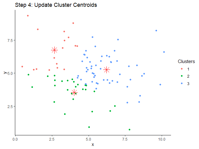
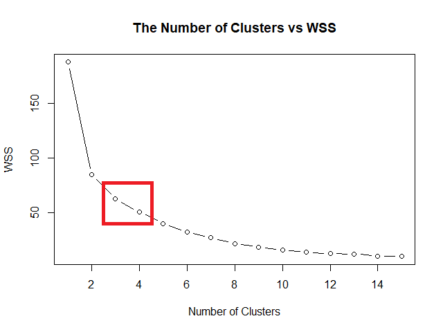
Elbow method หาค่า k ที่ดีที่สุด โดยสร้างกราฟระหว่างค่า k และ within-cluster sum of squares (WSS) หรือระยะห่างระหว่างข้อมูลในกลุ่ม ค่า k ที่ดีที่สุด คือ ค่า k ที่ WSS เริ่มไม่ลดลง

ในภาษา R เราสามารถเริ่มสร้างกราฟได้ โดยเริ่มจากใช้ for loop หา WSS สำหรับช่วงค่า k ที่เราต้องการ

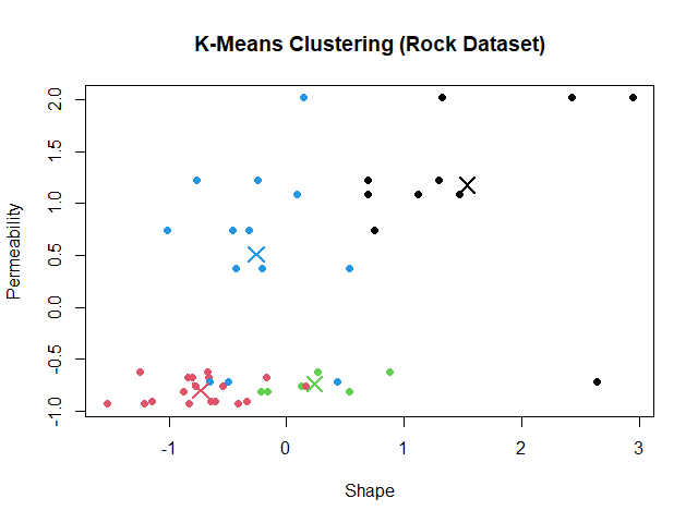
ในตัวอย่าง rock dataset เราจะใช้ช่วงค่า k ระหว่าง 1 ถึง 15:

# Initialise a vector for within cluster sum of squares (wss)
wss <- numeric(15)

# For-loop through the wss
for (k in 1:15) {
  
  ## Try the k
  km <- kmeans(rock_scaled,
               centers = k,
               nstart = 20)
  
  ## Get WSS for the k
  wss[k] <- km$tot.withinss
}

จากนั้น ใช้ plot() สร้างกราฟความสัมพันธ์ระหว่างค่า k และ WSS:

# Plot the wss
plot(1:15,
     wss,
     type = "b",
     main = "The Number of Clusters vs WSS",
     xlab = "Number of Clusters",
     ylab = "WSS")

ผลลัพธ์:

จากกราฟ จะเห็นว่า WSS เริ่มชะลอตัว เมื่อค่า k อยู่ที่ 3 และ 4 ซึ่งเป็นจุดที่เป็นข้อศอก (elbow) ของกราฟ:

แสดงว่า optimal k มีค่า 3 หรือ 4

สำหรับบทความนี้ เราจะกำหนด optimal k = 4:

# Set optiomal k = 4
opt_k <- 4

⏹️ k-Means

🔥 Train the Model

หลังเตรียมข้อมูลและหา optimal k แล้ว เราก็พร้อมที่จะใช้ kmeans() ในการจัดกลุ่มข้อมูลแล้ว:

# Set see for reproducibility
set.seed(100)

# Train the model
km <- kmeans(rock_scaled,
             centers = opt_k,
             nstart = 20)

🤓 Get the Results

เราสามารถดูผลการจัดกลุ่มได้ 2 วิธี:

วิธีที่ 1. ดูค่าทางสถิติ:

# Print the model
print(km)

ผลลัพธ์:

K-means clustering with 4 clusters of sizes 10, 18, 6, 14

Cluster means:
        area       peri
1 -0.4406840 -0.9164442
2  0.3496197  0.8022501
3  1.5646450  1.3101981
4 -0.8052989 -0.9383748
       shape       perm
1  1.5369800  1.1775435
2 -0.7319607 -0.8017914
3  0.2358392 -0.7425075
4 -0.2578245  0.5079897

Clustering vector:
 [1] 2 2 2 2 2 2 2 2 2 2 2 2 3
[14] 2 2 2 3 3 3 2 2 3 3 2 1 4
[27] 4 4 4 1 1 1 4 1 4 1 4 1 4
[40] 4 1 4 1 1 4 4 4 4

Within cluster sum of squares by cluster:
[1] 18.917267  8.104718
[3]  1.471788 22.095636
 (between_SS / total_SS =  73.1 %)

Available components:

[1] "cluster"     
[2] "centers"     
[3] "totss"       
[4] "withinss"    
[5] "tot.withinss"
[6] "betweenss"   
[7] "size"        
[8] "iter"        
[9] "ifault"

จากผลลัพธ์ จะเห็นได้ว่า ข้อมูลถูกแบ่งเป็น 4 กลุ่ม และเราสามารถดูค่า mean และ WSS ของแต่ละกลุ่มได้

วิธีที่ 2. สร้างกราฟ:

# Create a plot
plot(rock_scaled[, c("shape", "perm")], 
     col = km$cluster,
     pch = 19,
     main = "K-Means Clustering (Rock Dataset)",
     xlab = "Shape",
     ylab = "Permeability")

# Add cluster centers
points(km$centers[, c("shape", "perm")], 
       col = 1:5,
       pch = 4,
       cex = 2,
       lwd = 2)

ผลลัพธ์:

ตอนนี้ เราก็ได้ข้อมูลที่จัดกลุ่มด้วย k-means เรียบร้อยแล้ว 👍

😺 GitHub

ดู code ทั้งหมดในบทความนี้ได้ที่ GitHub

📃 References

✅ R Book for Psychologists: หนังสือภาษา R สำหรับนักจิตวิทยา

📕 ขอฝากหนังสือเล่มแรกในชีวิตด้วยนะครับ 😆

🙋 ใครที่กำลังเรียนจิตวิทยาหรือทำงานสายจิตวิทยา และเบื่อที่ต้องใช้ software ราคาแพงอย่าง SPSS และ Excel เพื่อทำข้อมูล

💪 ผมขอแนะนำ R Book for Psychologists หนังสือสอนใช้ภาษา R เพื่อการวิเคราะห์ข้อมูลทางจิตวิทยา ที่เขียนมาเพื่อนักจิตวิทยาที่ไม่เคยมีประสบการณ์เขียน code มาก่อน

ในหนังสือ เราจะปูพื้นฐานภาษา R และพาไปดูวิธีวิเคราะห์สถิติที่ใช้บ่อยกัน เช่น:

Correlation
t-tests
ANOVA
Reliability
Factor analysis

🚀 เมื่ออ่านและทำตามตัวอย่างใน R Book for Psychologists ทุกคนจะไม่ต้องพึง SPSS และ Excel ในการทำงานอีกต่อไป และสามารถวิเคราะห์ข้อมูลด้วยตัวเองได้ด้วยความมั่นใจ

แล้วทุกคนจะแปลกใจว่า ทำไมภาษา R ง่ายขนาดนี้ 🙂‍↕️

👉 สนใจดูรายละเอียดหนังสือได้ที่ meb:

ดูรายละเอียดหนังสือ R Book for Psychologists

2025-05-01

สอนปลูกต้นไม้ในภาษา R (ภาค 1): วิธีสร้าง tree-based models ใน 3 ขั้นตอนด้วย rpart และ randomForest packages — ตัวอย่างการทำนายประเภทเกียร์รถใน mtcars dataset

ในบทความนี้ เราจะมาทำความรู้จักและสร้าง tree-based models ในภาษา R กัน:

Classification tree
Random forest

ถ้าพร้อมแล้ว ไปเริ่มกันเลย

🌳 Tree-Based Algorithms คืออะไร?

Tree-based algorithm เป็น machine learning algorithm ประเภท supervised learning ที่ทำนายข้อมูลโดยใช้ decision tree

Decision tree เป็นเครื่องมือช่วยตัดสินใจที่ดูคล้ายกับต้นไม้กลับหัว เพราะประกอบด้วยจุดตัดสินใจ (node) ที่แตกยอด (ทางเลือก) ออกไปเรื่อย ๆ เพื่อใช้ทำนายผลลัพธ์ที่ต้องการ

ยกตัวอย่างเช่น เราอยากรู้ว่า เราควรจะสมัครงานกับบริษัทแห่งหนึ่งไหม เราอาจจะสร้าง decision tree จาก 3 ปัจจัย คือ:

เงินเดือน
ได้ใช้ทักษะที่มี
การทำงานแบบ hybrid หรือ remote

ได้แบบนี้:

จาก decision tree ถ้าเราเห็นงานที่ได้เงินเดือนไม่ตรงใจ เราจะไม่สมัครงานนั้น (เส้นการตัดสินใจซ้ายสุด)

ในทางกลับกัน ถ้างานมีเงินเดือนที่น่าสนใจ และได้ใช้ทักษะที่มีอยู่ เราจะสมัครงานนั้น (เส้นการตัดสินใจขวาสุด) เป็นต้น

💻 Tree-Based Models ในภาษา R

ในภาษา R เราสามารถสร้าง tree-based model ได้ด้วย rpart() จาก rpart package:

# Install
install.packages("rpart")
# Load
library(rpart)

rpart() ต้องการ 4 arguments ดังนี้:

rpart(formula, data, method, control)

formula = สูตรในการวิเคราะห์ (ตัวแปรตาม ~ ตัวแปรต้น)
data = dataset ที่ใช้สร้าง model
method = ประเภท algorithm ("anova" สำหรับ regression และ "class" สำหรับ classification)
control (optional) = เงื่อนไขควบคุม “การเติบโต” ของ decision tree เช่น ระดับชั้นที่มีได้ เป็นต้น

(Note: ศึกษาการใช้งาน rpart() เพิ่มเติมได้ที่ rpart: Recursive Partitioning and Regression Trees)

เราไปดูตัวอย่างการใช้งาน rpart() กัน

🚗 Dataset: mtcars

ในบทความนี้ เราจะลองสร้าง tree-based model ประเภท classification หรือ classification tree เพื่อทำนายประเภทเกียร์รถใน mtcars dataset

mtcars เป็นชุดข้อมูลรถจาก ปี ค.ศ. 1974 ซึ่งประกอบไปด้วยข้อมูล เช่น รุ่นรถ น้ำหนัก ระดับการกินน้ำมัน แรงม้า เป็นต้น

เราสามารถโหลด mtcars มาใช้งานได้ด้วย data() และ preview ด้วย head():

# Load
data(mtcars)
# Preview
head(mtcars)

ตัวอย่างข้อมูล:

                   mpg cyl disp  hp drat    wt  qsec vs        am gear carb
Mazda RX4         21.0   6  160 110 3.90 2.620 16.46  0    manual    4    4
Mazda RX4 Wag     21.0   6  160 110 3.90 2.875 17.02  0    manual    4    4
Datsun 710        22.8   4  108  93 3.85 2.320 18.61  1    manual    4    1
Hornet 4 Drive    21.4   6  258 110 3.08 3.215 19.44  1 automatic    3    1
Hornet Sportabout 18.7   8  360 175 3.15 3.440 17.02  0 automatic    3    2
Valiant           18.1   6  225 105 2.76 3.460 20.22  1 automatic    3    1

🔧 Prepare the Data

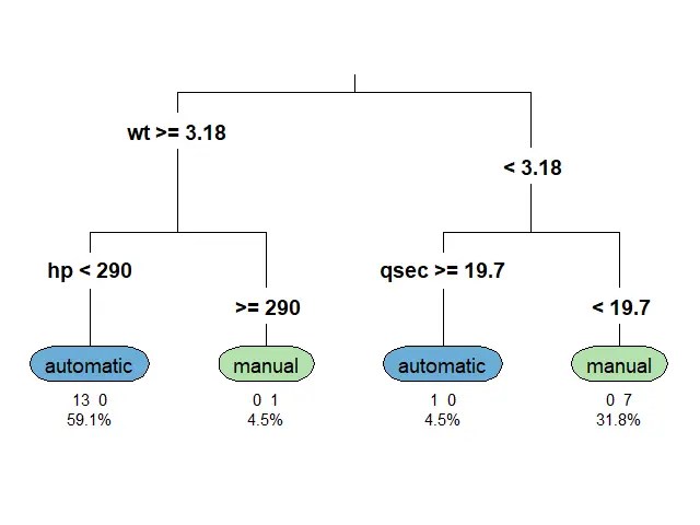
ก่อนนำ mtcars ไปใช้สร้าง classification tree เราจะต้องทำ 2 อย่างก่อน:

อย่างที่ #1. ปรับ column am ให้เป็น factor เพราะสิ่งที่เราต้องการทำนายเป็น categorical data:

# Convert `am` to factor
mtcars$am <- factor(mtcars$am,
                    levels = c(0, 1),
                    labels = c("automatic", "manual"))
# Check the result
class(mtcars$am)

ผลลัพธ์:

[1] "factor"

อย่างที่ #2. Split ข้อมูลเป็น 2 ชุด:

Training set สำหรับสร้าง model
Test set สำหรับประเมิน model

# Set seed for reproducibility
set.seed(500)
# Get training index
train_index <- sample(nrow(mtcars),
                      nrow(mtcars) * 0.7)
# Split the data
train_set <- mtcars[train_index, ]
test_set <- mtcars[-train_index, ]

🪴 Train the Model

ตอนนี้ เราพร้อมที่จะสร้าง classification tree ด้วย rpart() แล้ว

สำหรับ classification tree ในบทความนี้ เราจะลองตั้งเงื่อนไขในการปลูกต้นไม้ (control) ดังนี้:

Argument	Explanation
`cp = 0`	คะแนนประสิทธิภาพขั้นต่ำ ก่อนจะแตกกิ่งใหม่ได้ = 0
`minsplit = 1`	จำนวนกิ่งย่อยขั้นต่ำที่ต้องมี ก่อนจะแตกกิ่งใหม่ได้ = 1
`maxdepth = 5`	จำนวนชั้นที่ decision tree มีได้สูงสุด = 5

# Classification tree
ct <- rpart(am ~ .,
            data = train_set,
            method = "class",
            control = rpart.control(cp = 0, minsplit = 1, maxdepth = 5))

เราสามารถดู classification tree ของเราได้ด้วย rpart.plot():

# Plot classification tree
rpart.plot(ct,
           type = 3,
           extra = 101,
           under = TRUE,
           digits = 3,
           tweak = 1.2)

ผลลัพธ์:

Note:

ก่อนใช้งาน rpart.plot() เราต้องจะติดตั้งและเรียกใช้งานด้วย install.packages() และ library() ตามลำดับ
ศึกษาการใช้งาน rpart.plot() เพิ่มเติมได้ที่ rpart.plot: Plot an rpart model. A simplified interface to the prp function.

📏 Evaluate the Model

เมื่อได้ classification tree มาแล้ว เราลองมาประเมินความสามารถของ model ด้วย accuracy หรือสัดส่วนการทำนายที่ถูกต้องกัน

เราเริ่มจากใช้ predict() เพื่อใช้ model ทำนายประเภทเกียร์:

# Predict the outcome
test_set$pred_ct <- predict(ct,
                            newdata = test_set,
                            type = "class")

จากนั้น สร้าง confusion matrix หรือ matrix เปรียบเทียบคำทำนายกับข้อมูลจริง:

# Create a confusion matrix
cm_ct <- table(Predicted = test_set$pred_ct,
               Actual = test_set$am)
# Print confusion matrix
print(cm_ct)

ผลลัพธ์:

           Actual
Predicted   automatic manual
  automatic         5      1
  manual            0      4

สุดท้าย เราหา accuracy ด้วยการนำจำนวนคำทำนายที่ถูกต้องมาหารด้วยจำนวนคำทำนายทั้งหมด:

# Get accuracy
acc_ct <- sum(diag(cm_ct)) / sum(cm_ct)
# Print accuracy
cat("Accuracy (classification tree):", acc_ct)

ผลลัพธ์:

Accuracy (classification tree): 0.9

จะเห็นได้ว่า model ของเรามีความแม่นยำถึง 90%

🍄 Random Forest

Random forest เป็น tree-based algorithm ที่ช่วยเพิ่มความแม่นยำในการทำนาย โดยสุ่มสร้าง decision trees ต้นเล็กขึ้นมาเป็นกลุ่ม (forest) แทนการปลูก decision tree ต้นเดียว

Decision tree แต่ละต้นใน random forest มีความสามารถในการทำนายแตกต่างกัน ซึ่งบางต้นอาจมีความสามารถที่น้อยมาก

แต่จุดแข็งของ random forest อยู่ที่จำนวน โดย random forest ทำนายผลลัพธ์โดยดูจากผลลัพธ์ในภาพรวม ดังนี้:

Task	Predict by
Regression	ค่าเฉลี่ยของผลลัพธ์การทำนายของทุกต้น
Classification	เสียงส่วนมาก (majority vote)

ดังนั้น แม้ว่า decision tree บางต้นอาจทำนายผิดพลาด แต่โดยรวมแล้ว random forest มีโอกาสที่จะทำนายได้ดีกว่า decision tree ต้นเดียว

ในภาษา R เราสามารถสร้าง random forest ได้ด้วย randomForest() จาก randomForest package ซึ่งต้องการ 3 arguments:

randomFrest(formula, data, ntree)

formula = สูตรในการวิเคราะห์ (ตัวแปรตาม ~ ตัวแปรต้น)
data = dataset ที่ใช้สร้าง model
ntree = จำนวน decision trees ที่ต้องการสร้าง

Note:

เราไม่ต้องกำหนดว่า จะทำ classification หรือ regression model เพราะ randomForest() จะเลือก model ให้อัตโนมัติตามข้อมูลที่เราใส่เข้าไป
ศึกษาการใช้งาน randomForest() เพิ่มเติมได้ที่ randomForest: Classification and Regression with Random Forest

ก่อนใช้ randomForest() เราต้องเตรียมข้อมูลแบบเดียวกันกับ rpart() ได้แก่:

เปลี่ยน am ให้เป็น factor
Split the data

สมมุติว่า เราเตรียมข้อมูลแล้ว เราสามารถเรียกใช้ randomForest() ได้เลย โดยเราจะลองสร้าง random forest ที่ประกอบด้วย decision trees 100 ต้น:

# Random forest
rf <- randomForest(am ~ .,
                   data = train_set,
                   ntree = 100)

แล้วลองประเมินความสามารถของ model ด้วย accuracy

เริ่มจากทำนายประเภทเกียร์:

# Predict the outcome
test_set$pred_rf <- predict(rf,
                            newdata = test_set,
                            type = "class")

สร้าง confusion matrix:

# Create a confusion matrix
cm_rf <- table(Predicted = test_set$pred_rf,
               Actual = test_set$am)
# Print confusion matrix
print(cm_rf)

ผลลัพธ์:

           Actual
Predicted   automatic manual
  automatic         5      0
  manual            0      5

และสุดท้าย คำนวณ accuracy:

# Get accuracy
acc_rf <- sum(diag(cm_rf)) / sum(cm_rf)
# Print accuracy
cat("Accuracy (random forest):", acc_rf)

ผลลัพธ์:

Accuracy (random forest): 1

จะเห็นว่า random forest (100%) มีความแม่นยำในการทำนายมากกว่า classification tree ต้นเดียว (90%)

🐱 GitHub

ดู code ทั้งหมดในบทความนี้ได้ที่ GitHub:

📃 References

✅ R Book for Psychologists: หนังสือภาษา R สำหรับนักจิตวิทยา

📕 ขอฝากหนังสือเล่มแรกในชีวิตด้วยนะครับ 😆

Correlation
t-tests
ANOVA
Reliability
Factor analysis

แล้วทุกคนจะแปลกใจว่า ทำไมภาษา R ง่ายขนาดนี้ 🙂‍↕️

👉 สนใจดูรายละเอียดหนังสือได้ที่ meb:

ดูรายละเอียดหนังสือ R Book for Psychologists

2025-04-24

วิธีสร้าง Naïve Bayes classifier ใน 5 ขั้นตอนด้วย naivebayes package ในภาษา R – ตัวอย่างการทำนายประเภทดอกไม้ใน iris dataset
ในบทความนี้ เราจะมาทำความรู้กับ Naïve Bayes และดูวิธีสร้าง Naïve Bayes classifier ในภาษา R ด้วย naivebayes package กัน
👼 Naïve Bayes คืออะไร?

Naïve Bayes (NB) เป็น machine learning algorithm ประเภท supervised learning สำหรับทำนายกลุ่มของข้อมูล (classification)

NB ทำนายข้อมูล โดยวิเคราะห์ความน่าจะเป็นที่ 2 เหตุการณ์ (ตัวแปรต้นและตัวแปรตาม) จะเกิดขึ้นคู่กัน

ยกตัวอย่างเช่น การอนุมัติสินเชื่อ (อนุมัติ/ไม่อนุมัติ) ที่เกิดขึ้นอยู่กับ:
- รายได้: รายได้มาก -> อนุมัติ
- อายุ: อายุน้อย -> อนุมัติ
- ประวัติการขอสินเชื่อ: เคยขอแล้วผ่าน -> อนุมัติ
NB คำนวณความน่าจะเป็นของแต่ละปัจจัยต่อตัวแปรตาม (การอนุมัติ) โดยอนุมานว่า แต่ละปัจจัยเกิดแยกกัน (independent) แม้ว่าในความเป็นจริงหลายปัจจัยจะเกิดขึ้นร่วมกัน (dependent; เช่น อายุมาก -> รายได้มาก) ก็ตาม

เนื่องจาก NB มีการมองโลกอย่างง่าย จึงได้ชื่อว่า “naïve” หรือไร้เดียงนั่นเอง

แม้ว่า NB จะมีการมองโลกที่ไร้เดียงสา แต่ก็เป็น algorithm ที่:
1. เข้าใจได้ง่าย (เพราะไร้เดียงสา)
2. รวดเร็ว (เพราะใช้การวิเคราะห์อย่างง่าย)
3. น่าเชื่อถือ (มักจะทำนายได้แม่นยำ แม้จะมีมุมมองที่ไม่ตรงกับความเป็นจริง)
🧑‍💻 วิธีสร้าง NB Classifer ด้วย naivebayes Package

วิธีการสร้าง NB classifier ด้วย naivebayes package มี 5 ขั้นตอน ได้แก่:
1. Install and load the package
2. Load and preview the dataset
3. Split the dataset
4. Create a NB model
5. Evaluate the model
.

1️⃣ Step 1. Install & Load the Package

ในขั้นแรก เราต้องติดตั้งและเรียกใช้งาน naivebayes package:
```
# Install and load the package
## Install
install.packages("naivebayes")
## Load
library(naivebayes)
```
Note: เราทำการติดตั้งแค่ครั้งแรกครั้งเดียว แต่การเรียกใช้ต้องทำทุกครั้งทุกเริ่ม session ใหม่

.

2️⃣ Step 2. Load & Preview the Dataset

ในขั้นที่สอง ให้เราโหลด dataset ที่จะใช้งาน

โดยในบทความนี้ เราจะใช้ built-in dataset ในภาษา R ชื่อ iris dataset

iris dataset มีกลีบดอกของข้อมูลดอกไม้ 3 ชนิด ได้แก่:
- Iris setosa
- Iris virginica
- Iris versicolor
เป้าหมายของเรา คือ ทำนายประเภทของดอกไม้จากความกว้างและความยาวกลีบดอก

เนื่องจากเป็น built-in dataset เราสามารถโหลด iris dataset ด้วยคำสั่ง data():
```
# Load
data(iris)
```
จากนั้น เราสามารถใช้คำสั่ง head() เพื่อ preview ข้อมูล:
```
# Preview
head(iris)
```
ผลลัพธ์:
```
  Sepal.Length Sepal.Width Petal.Length Petal.Width Species
1          5.1         3.5          1.4         0.2  setosa
2          4.9         3.0          1.4         0.2  setosa
3          4.7         3.2          1.3         0.2  setosa
4          4.6         3.1          1.5         0.2  setosa
5          5.0         3.6          1.4         0.2  setosa
6          5.4         3.9          1.7         0.4  setosa
```
Note: จะเห็นว่า iris dataset มีข้อมูลทั้งหมด 5 columns คือ ความยาวและความกว้างของกลีบดอกชั้นนอก (sepal) และความยาวและความกว้างของกลีบดอกชั้นใน (petal) รวมทั้งประเภทดอกไม้ (species)

เนื่องจาก NB classifier ต้องการตัวแปรตามที่เป็น factor เราต้องเช็กได้ว่า Species เป็น data type ไหนด้วยคำสั่ง str():
```
# Preview
str(iris)
```
ผลลัพธ์:
```
'data.frame':	150 obs. of  5 variables:
 $ Sepal.Length: num  5.1 4.9 4.7 4.6 5 5.4 4.6 5 4.4 4.9 ...
 $ Sepal.Width : num  3.5 3 3.2 3.1 3.6 3.9 3.4 3.4 2.9 3.1 ...
 $ Petal.Length: num  1.4 1.4 1.3 1.5 1.4 1.7 1.4 1.5 1.4 1.5 ...
 $ Petal.Width : num  0.2 0.2 0.2 0.2 0.2 0.4 0.3 0.2 0.2 0.1 ...
 $ Species     : Factor w/ 3 levels "setosa","versicolor",..: 1 1 1 1 1 1 1 1 1 1 ...
```
จะเห็นได้ว่า Species เป็น factor อยู่แล้ว และพร้อมที่ใช้สร้าง NB classifier

.

3️⃣ Step 3. Split the Dataset

ในขั้นที่สาม เราจะแบ่งข้อมูลเป็น 2 ชุด:
1. Training set เพื่อสร้าง NB classifier
2. Test set เพื่อทดสอบประสิทธิภาพของ NB classifier
ขั้นแรกในการแบ่งข้อมูล ให้เราสุ่มเลือก row index ที่จะอยู่ใน training set:
```
# Set seed for reproducibility
set.seed(2025)
# Create a training index
training_index <- sample(1:nrow(iris),
                         0.7 * nrow(iris))
```
จากนั้น ใช้ row index ที่ได้แบ่งข้อมูลเป็น 2 ชุด:
```
# Split the dataset
train_set <- iris[training_index, ]
test_set <- iris[-training_index, ]
```
.

4️⃣ Step 4. Create a NB Model

ในขั้นที่สี่ เราจะสร้าง NB classifier โดยใช้ naive_bayes() จาก naivebayes package

naive_bayes() ต้องการ input 2 อย่าง:
1. Formula: ตัวแปรต้นและตัวแปรตามที่ต้องการใช้สร้าง model โดยในกรณีนี้ คือ ทำนาย Species ด้วยข้อมูลที่เหลือทั้งหมด (.)
2. Data: dataset ที่จะใช้สร้าง model ซึ่งในกรณีนี้ คือ train_set
```
# Create a NB model
nb <- naive_bayes(Species ~ .,
                  data = train_set)
```
เมื่อเราได้ NB classifier มาแล้ว เรามาลองใช้ model ทำนายประเภทดอกไม้กัน:
```
# Predict the outcomes
pred <- predict(nb,
                newdata = test_set[, 1:4],
                type = "class")
print(pred)
```
ผลลัพธ์:
```
 [1] setosa     setosa     setosa     setosa     setosa    
 [6] setosa     setosa     setosa     setosa     setosa    
[11] setosa     setosa     setosa     setosa     setosa    
[16] virginica  versicolor versicolor versicolor versicolor
[21] virginica  versicolor versicolor versicolor versicolor
[26] versicolor virginica  versicolor versicolor versicolor
[31] versicolor versicolor versicolor versicolor virginica 
[36] virginica  virginica  virginica  virginica  virginica 
[41] virginica  virginica  virginica  virginica  virginica 
Levels: setosa versicolor virginica
```
.

5️⃣ Step 5. Evaluate the Model

ในขั้นสุดท้าย เราจะประเมินประสิทธิภาพของ model ด้วยการคำนวณ accuracy หรือ สัดส่วนของคำตอบที่ model ตอบถูก:

Accuracy = Correct predictions / Total predictions

เราสามารถหาค่า accuracy ได้โดยเริ่มสร้าง confusion matrix ก่อน:
```
# Create a confusion matrix
cm <- table(Predicted = pred, 
            Actual = test_set$Species)
print(cm)
```
ผลลัพธ์:
```
            Actual
Predicted    setosa versicolor virginica
  setosa         15          0         0
  versicolor      0         16         0
  virginica       0          3        11
```
จากนั้น นำจำนวนคำตอบที่ถูกต้องและจำนวนคำตอบทั้งหมดมาหาค่า accuracy:
```
# Calculate the accuracy
accuracy <- sum(diag(cm)) / sum(cm)
cat("Accuracy:", round(accuracy, 2))
```
ผลลัพธ์:
```
Accuracy: 0.93
```
จะเห็นได้ว่า NB classifier ที่เป็น model ไร้เดียงสาของเรา มีความแม่นยำในการทำนายสูงถึง 93%

😺 GitHub

ดู code ทั้งหมดในบทความนี้ได้ที่ GitHub

📃 References
✅ R Book for Psychologists: หนังสือภาษา R สำหรับนักจิตวิทยา

📕 ขอฝากหนังสือเล่มแรกในชีวิตด้วยนะครับ 😆

🙋 ใครที่กำลังเรียนจิตวิทยาหรือทำงานสายจิตวิทยา และเบื่อที่ต้องใช้ software ราคาแพงอย่าง SPSS และ Excel เพื่อทำข้อมูล

💪 ผมขอแนะนำ R Book for Psychologists หนังสือสอนใช้ภาษา R เพื่อการวิเคราะห์ข้อมูลทางจิตวิทยา ที่เขียนมาเพื่อนักจิตวิทยาที่ไม่เคยมีประสบการณ์เขียน code มาก่อน

ในหนังสือ เราจะปูพื้นฐานภาษา R และพาไปดูวิธีวิเคราะห์สถิติที่ใช้บ่อยกัน เช่น:
- Correlation
- t-tests
- ANOVA
- Reliability
- Factor analysis
🚀 เมื่ออ่านและทำตามตัวอย่างใน R Book for Psychologists ทุกคนจะไม่ต้องพึง SPSS และ Excel ในการทำงานอีกต่อไป และสามารถวิเคราะห์ข้อมูลด้วยตัวเองได้ด้วยความมั่นใจ

แล้วทุกคนจะแปลกใจว่า ทำไมภาษา R ง่ายขนาดนี้ 🙂‍↕️

👉 สนใจดูรายละเอียดหนังสือได้ที่ meb:

ดูรายละเอียดหนังสือ R Book for Psychologists
Share this:
X
Facebook
Like Loading…
2025-04-10
วิธีสร้าง KNN model ใน 5 ขั้นตอนด้วย class package ในภาษา R – ตัวอย่างการทำนายประเภทดอกไม้ใน iris dataset
ในบทความนี้ เราจะมาทำความรู้กันกับ KNN model และวิธีสร้าง KNN model ด้วย class package ในภาษา R กัน
KNN หรือ K-Nearest Neighbors เป็น machine learning algorithm ประเภท supervised learning ซึ่งใช้ได้กับงานประเภท classification (จัดกลุ่ม) และ regression (ทำนายแนวโน้ม)

การทำงานของ KNN ตรงไปตรงมา คือ ทำนายข้อมูลโดยการดูจากข้อมูลใกล้เคียง จำนวน k ข้อมูล (เราสามารถกำหนดค่า k เองได้)

ยกตัวอย่างเช่น เราต้องการใช้ KNN ทำนายราคาหุ้น KNN จะดูราคาหุ้นที่อยู่ใกล้เคียงกับหุ้นที่เราต้องการทำนายราคา เช่น 5 หุ้นใกล้เคียง โดย:
- 2/5 หุ้น = ราคาลง
- 3/5 หุ้น = ราคาขึ้น
KNN จะทำนายว่า หุ้นในใจของเรา จะราคาขึ้น เพราะหุ้นใกล้เคียงส่วนใหญ่ปรับราคาขึ้น เป็นต้น

💻 KNN in R With class Package

เราสามารถสร้าง KNN model ในภาษา R ด้วย class package โดยมี 5 ขั้นตอนดังนี้:
1. Get class package
2. Load the dataset
3. Prepare the data
4. Train a KNN model
5. Evaluate the model
เราไปดูตัวอย่างการสร้าง KNN model เพื่อทำนายประเภทดอกไม้ ด้วย iris dataset กัน

1️⃣ Step 1. Get class Package

ในขั้นแรก ให้เราติดตั้งและเรียกใช้งาน class package

ติดตั้ง (ทำครั้งเดียว):
```
# Install
install.packages("class")
```
เรียกใช้งาน (ทำทุกครั้งที่เริ่ม session ใหม่):
```
# Load
library(class)
```
2️⃣ Step 2. Get the Dataset

ในขั้นที่สอง ให้เราโหลด dataset ที่จะใช้งาน

โดยในบทความนี้ เราจะใช้ iris ที่มีข้อมูลดอกไม้ 3 ชนิด ได้แก่:
- Iris setosa
- Iris virginica
- Iris versicolor
นอกจากประเภทดอกไม้ (species) iris dataset ยังประกอบด้วยความกว้าง (width) และความยาว (length) ของกลีบดอกชั้นนอก (sepal) และชั้นใน (petal)

เนื่องจาก iris เป็น built-in dataset ใน ภาษา R เราสามารถโหลดข้อมูลด้วยคำสั่ง data() ได้:
```
# Load
data(iris)
```
เมื่อโหลดแล้ว เราสามารถดูตัวอย่าง dataset ได้ด้วย head():
```
# Preview
head(iris)
```
ผลลัพธ์:
```
  Sepal.Length Sepal.Width Petal.Length Petal.Width Species
1          5.1         3.5          1.4         0.2  setosa
2          4.9         3.0          1.4         0.2  setosa
3          4.7         3.2          1.3         0.2  setosa
4          4.6         3.1          1.5         0.2  setosa
5          5.0         3.6          1.4         0.2  setosa
6          5.4         3.9          1.7         0.4  setosa
```
3️⃣ Step 3. Prepare Data

ในขั้นที่สาม เราจะเตรียมข้อมูล เพื่อใช้สร้าง KNN model

โดยสำหรับ iris dataset เราจะทำ 3 อย่าง คือ:
1. Normalise data
2. Split data
3. Separate features from the label
.

📉 Normalise Data

เนื่องจาก KNN model อ้างอิงระยะห่างระหว่างข้อมูลในการทำนายผลลัพธ์ ข้อมูลที่มีช่วงกว้าง (เช่น 0-100) จะมีน้ำหนักกว่าข้อมูลที่มีช่วงแคบ (เช่น 0-10) และทำให้ model ของเรา bias ได้

เพื่อป้องกันความเสี่ยงนี้ เราต้อง normalise ข้อมูล หรือการทำให้ข้อมูลมีช่วงมีช่วงข้อมูลเดียวกัน

การทำ normalisation มีหลายวิธี แต่วิธีที่นิยมใช้กับ KNN คือ min-max normalisation ซึ่งเปลี่ยนช่วงข้อมูลให้อยู่ในช่วง 0-1 ผ่านสูตร:
```
(X - Min) / (Max - Min)
```
- X คือ ข้อมูล
- Min คือ ค่าที่น้อยที่สุด
- Max คือ ค่าที่มากที่สุด
ในภาษา R เราไม่มี function ที่ใช้ทำ min-max normalisation ได้โดยตรง เราเลยต้องเขียน function ขึ้นมาใช้เอง:
```
# Define a function for normalisation
normalise <- function(x) {
  return((x - min(x)) / (max(x) - min(x)))
}
```
จากนั้น ให้เราใช้ function นี้กับ columns ที่เป็นตัวเลข (numeric) เช่น Sepal.Length แล้วเก็บผลลัพธ์ไว้ใน data frame ใหม่ ชื่อ iris_normalises:
```
# Apply the function to the dataset
iris_normalised <- as.data.frame(lapply(iris[, 1:4],
                                        normalise))
```
เนื่องจากตอนที่เราใช้ function เราตัด column ที่ไม่ใช่ตัวเลขออก ทำให้ iris_normalised ไม่มี column Species

เราสามารถใส่ Species กลับเข้าไป เพื่อใช้ในขั้นตอนถัดไป แบบนี้:
```
# Add species column back into the data frame
iris_normalised$Species <- iris$Species
```
สุดท้าย เราเช็กผลลัพธ์ด้วยการเรียกดูสถิติของ iris_normalised:
```
# Check the results
summary(iris_normalised)
```
ผลลัพธ์:
```
  Sepal.Length     Sepal.Width    
 Min.   :0.0000   Min.   :0.0000  
 1st Qu.:0.2222   1st Qu.:0.3333  
 Median :0.4167   Median :0.4167  
 Mean   :0.4287   Mean   :0.4406  
 3rd Qu.:0.5833   3rd Qu.:0.5417  
 Max.   :1.0000   Max.   :1.0000  
  Petal.Length     Petal.Width     
 Min.   :0.0000   Min.   :0.00000  
 1st Qu.:0.1017   1st Qu.:0.08333  
 Median :0.5678   Median :0.50000  
 Mean   :0.4675   Mean   :0.45806  
 3rd Qu.:0.6949   3rd Qu.:0.70833  
 Max.   :1.0000   Max.   :1.00000  
       Species  
 setosa    :50  
 versicolor:50  
 virginica :50  
```
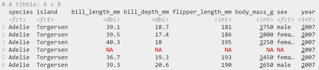
จะเห็นว่า:
1. Columns ที่เป็นตัวเลข มีช่วงอยู่ระหว่าง 0 และ 1
2. เรายังมี column Species อยู่
.

🪓 Split Data

ในการสร้าง KNN model เราควรแบ่ง dataset ที่มีเป็น 2 ส่วน คือ:
1. Training set: ใช้สำหรับสร้าง model
2. Test set: ใช้สำหรับประเมิน model
เราเริ่มแบ่งข้อมูลด้วยการสุ่ม row index ที่จะอยู่ใน training set:
```
# Set seed for reproducibility
set.seed(2025)

# Create a training index
train_index <- sample(1:nrow(iris_normalised),
                      0.7 * nrow(iris_normalised))
```
จากนั้น subset ข้อมูลด้วย row index ที่สุ่มไว้:
```
# Split the data
train_set <- iris_normalised[train_index, ]
test_set <- iris_normalised[-train_index, ]
```
.

🏷️ Separate Features From Label

ขั้นตอนสุดท้ายในการเตรียมข้อมูล คือ แยก features หรือ X (columns ที่จะใช้ทำนาย) ออกจาก label หรือ Y (สิ่งที่ต้องการทำนาย):
```
# Separate features from label

## Training set
train_X <- train_set[, 1:4]
train_Y <- train_set$Species

## Test set
test_X <- test_set[, 1:4]
test_Y <- test_set$Species
```
4️⃣ Step 4. Train a KNN Model

ขั้นที่สี่เป็นขั้นที่เราสร้าง KNN model ขึ้นมา โดยเรียกใช้ knn() จาก class package

ทั้งนี้ knn() ต้องการ input 3 อย่าง:
1. train: fatures จาก training set
2. test: feature จาก test set
3. cl: label จาก training set
4. k: จำนวนข้อมูลใกล้เคียงที่จะใช้ทำนายผลลัพธ์
```
# Train a KNN model
pred <- knn(train = train_X,
            test = test_X,
            cl = train_Y,
            k = 5)
```
ในตัวอย่าง เรากำหนด k = 5 เพื่อทำนายผลลัพธ์โดยดูจากข้อมูลที่ใกล้เคียง 5 อันดับแรก

5️⃣ Step 5. Evaluate the Model

หลังจากได้ model แล้ว เราประเมินประสิทธิภาพของ model ในการทำนายผลลัพธ์ ซึ่งเราทำได้ง่าย ๆ โดยคำนวณ accuracy หรือสัดส่วนของข้อมูลที่ model ตอบถูกต่อจำนวนข้อมูลทั้งหมด:
```
Accuracy = Correct predictions / Total predictions
```
ในภาษา R ให้เราสร้าง confusion matrix หรือ matrix แสดงจำนวนคำตอบที่ถูกและผิด ด้วย table() function:
```
# Create a confusion matrix
cm <- table(Predicted = predictions,
            Actual = test_Y)

# Print the matrix
print(cm)
```
ผลลัพธ์:
```
            Actual
Predicted    setosa versicolor virginica
  setosa         15          0         0
  versicolor      0         17         0
  virginica       0          2        11
```
Note: จะเห็นได้ว่า model เราตอบถูกเป็นส่วนใหญ่ (ราว 90%)

จากนั้น คำนวณ accuracy ด้วย sum() และ diag():
```
# Calculate accuracy
acc <- sum(diag(cm)) / sum(cm)

# Print accuracy
cat("Accuracy:", round(acc, 2))
```
ผลลัพธ์:
```
Accuracy: 0.96
```
จากผลลัพธ์ เราจะเห็นว่า model มีความแม่นยำสูงถึง 96%

🍩 Bonus: Fine-Tuning

ในบางครั้ง ค่า k ที่เราตั้งไว้ อาจไม่ได้ทำให้เราได้ KNN model ที่ดีที่สุด

แทนที่เราจะแทนค่า k ใหม่ไปเรื่อย ๆ เราสามารถใช้ for loop เพื่อหาค่า k ที่ทำให้เราได้ model ที่ดีที่สุดได้

ให้เราเริ่มจากสร้าง vector ที่มีค่า k ที่ต้องการ:
```
# Create a set of k values
k_values <- 1:20
```
และ vector สำหรับเก็บค่า accuracy ของค่า k แต่ละตัว:
```
# Createa a vector for accuracy results
accuracy_results <- numeric(length(k_values))
```
แล้วใช้ for loop เพื่อหาค่า accuracy ของค่า k:
```
# For-loop through the k values
for (i in seq_along(k_values)) {
  
  ## Set the k value
  k <- k_values[i]
  
  ## Create a KNN model
  predictions <- knn(train = train_X,
                     test = test_X,
                     cl = train_Y,
                     k = k)
  
  ## Create a confusion matrix
  cm <- table(Predicted = predictions,
              Actual = test_Y)
  
  ## Calculate accuracy
  accuracy_results[i] <- sum(diag(cm)) / sum(cm)
}

# Find the best k and the corresponding accuracy
best_k <- k_values[which.max(accuracy_results)]
best_accuracy <- max(accuracy_results)

# Print best k and accuracy
cat(paste("Best k:", best_k),
    paste("Accuracy:", round(best_accuracy, 2)),
    sep = "\n")
```
ผลลัพธ์:
```
Best k: 12
Accuracy: 0.98
```
แสดงว่า ค่า k ที่ดีที่สุด คือ 12 โดยมี accuracy เท่ากับ 98%

นอกจากนี้ เรายังสามารถสร้างกราฟ เพื่อช่วยทำความเข้าใจผลของค่า k ต่อ accuracy:
```
# Plot the results
plot(k_values,
     accuracy_results,
     type = "b",
     pch = 19,
     col = "blue",
     xlab = "Number of Neighbors (k)",
     ylab = "Accuracy",
     main = "KNN Model Accuracy for Different k Values")
grid()
```
ผลลัพธ์:

จะเห็นได้ว่า k = 12 ให้ accuracy ที่ดีที่สุด และ k = 20 ให้ accuracy ต่ำที่สุด ส่วนค่า k อื่น ๆ ให้ accuracy ในช่วง 93 ถึง 96%

😺 GitHub

ดู code ทั้งหมดในบทความนี้ได้ที่ GitHub

📃 References
✅ R Book for Psychologists: หนังสือภาษา R สำหรับนักจิตวิทยา

📕 ขอฝากหนังสือเล่มแรกในชีวิตด้วยนะครับ 😆

🙋 ใครที่กำลังเรียนจิตวิทยาหรือทำงานสายจิตวิทยา และเบื่อที่ต้องใช้ software ราคาแพงอย่าง SPSS และ Excel เพื่อทำข้อมูล

💪 ผมขอแนะนำ R Book for Psychologists หนังสือสอนใช้ภาษา R เพื่อการวิเคราะห์ข้อมูลทางจิตวิทยา ที่เขียนมาเพื่อนักจิตวิทยาที่ไม่เคยมีประสบการณ์เขียน code มาก่อน

ในหนังสือ เราจะปูพื้นฐานภาษา R และพาไปดูวิธีวิเคราะห์สถิติที่ใช้บ่อยกัน เช่น:
- Correlation
- t-tests
- ANOVA
- Reliability
- Factor analysis
🚀 เมื่ออ่านและทำตามตัวอย่างใน R Book for Psychologists ทุกคนจะไม่ต้องพึง SPSS และ Excel ในการทำงานอีกต่อไป และสามารถวิเคราะห์ข้อมูลด้วยตัวเองได้ด้วยความมั่นใจ

แล้วทุกคนจะแปลกใจว่า ทำไมภาษา R ง่ายขนาดนี้ 🙂‍↕️

👉 สนใจดูรายละเอียดหนังสือได้ที่ meb:

ดูรายละเอียดหนังสือ R Book for Psychologists
Share this:
X
Facebook
Like Loading…
2025-04-03
แนะนำ dtplyr: package เชื่อม dplyr และ data.table เพื่อการทำ data wrangling กับข้อมูลขนาดใหญ่ที่ง่ายและรวดเร็ว — ตัวอย่างจาก mtcars dataset
ในบทความนี้ เรามาความรู้จักกับ package ในภาษา R ที่เรียกว่า dtplyr กัน
🏎️ dtplyr คืออะไร?

dtplyr เป็น package ที่เชื่อม 2 libraries ยอดนิยมสำหรับ data wrangling เข้าด้วยกัน ได้แก่:

.

Library #1. dplyr ซี่งมี verb-based syntax ที่ใช้งานง่าย

เช่น จาก mtcars dataset เลือกรถเกียร์ manual (am == 1) ที่มี miles/gallon (mpg) ตั้งแต่ 20 ขึ้นไป โดยเรียงจากมากไปน้อย:
```
# dplyr
mtcars |>
  filter(am == 1 & mpg >= 20) |>
  select(model, mpg) |>
  arrange(desc(mpg))
```
Note: mtcars ถูกปรับให้มี column ชื่อ model (ดู code ในการเพิ่ม column ได้ใน GitHub)

.

Library #2. data.table ซึ่งมี syntax ที่เข้าใจยากกว่า:
```
# data.table
mtcars_dt[am == 1 & mpg >= 20, .(model, mpg)][order(-mpg)]
```
Note: mtcars_dt เป็น dataset ที่ถูกเปลี่ยนจาก data.frame เป็น data.table object เพื่อใช้งานกับ data.table

แต่มีจุดเด่น คือ ประมวลผลได้เร็ว เหมาะกับการทำงานกับ data ขนาดใหญ่

.

dtplyr เชื่อม dplyr เข้ากับ data.table โดยการแปล dplyr syntax ให้เป็น data.table syntax ทำให้เราทำงานได้ง่ายและรวดเร็ว

🧑‍💻 วิธีใช้ dytplyr

เราสามารถใช้ dtplyr ได้ใน 3 ขั้นตอนง่าย ๆ:
1. Install and load dtplyr
2. Create a lazy data.table
3. Execute the syntax
.

1️⃣ ขั้นที่ 1. Install & Load dtplyr

ในการใช้งาน dtplyr เราต้องเรียกใช้ dplyr ด้วยเสมอ

ดังนั้น ในการติดตั้ง เราต้องติดตั้งทั้ง dtplyr และ dplyr:
```
# Install
install.packages("dplyr")
install.packages("dtplyr")
```
เมื่อติดตั้งแล้ว ให้เราเรียกใช้งาน dtplyr และ dplyr ทุกครั้งที่เริ่ม session ในการทำงาน:
```
# Load
library(dplyr)
library(dtplyr)
```
Note: คู่มือการใช้ dtplyr แนะนำให้โหลด data.table ด้วย เพื่อใช้ functions ของ data.table ในการทำงาน

.

2️⃣ ขั้นที่ 2. Create a Lazy data.table

หลังเรียกใช้งาน dtplyr ให้เราสร้าง dataset ที่เป็น lazy data.table object ขึ้นมา เพื่อช่วยให้ dtplyr เปลี่ยนคำสั่งของ dplyr เป็นคำสั่งของ data.table ได้:
```
# Convert mtcars dataset into lazy data.table object
mtcars_ldt <- lazy_dt(mtcars)
```
.

3️⃣ ขั้นที่ 3. Execute the Syntax

ในขั้นสุดท้าย เราสามารถเริ่มทำงานโดยใช้ syntax ของ dplyr ได้เลย:
```
# Execute the syntax
mtcars_ldt |>
  filter(am == 1 & mpg >= 20) |>
  select(model, mpg) |>
  arrange(desc(mpg)) |>
  as.data.table()
```
ผลลัพธ์:
```
             model   mpg
            <char> <num>
 1: Toyota Corolla  33.9
 2:       Fiat 128  32.4
 3:    Honda Civic  30.4
 4:   Lotus Europa  30.4
 5:      Fiat X1-9  27.3
 6:  Porsche 914-2  26.0
 7:     Datsun 710  22.8
 8:     Volvo 142E  21.4
 9:      Mazda RX4  21.0
10:  Mazda RX4 Wag  21.0
```
จะสังเกตว่า ใน code บรรทัดสุดท้าย เราเพิ่ม as.data.table() เข้ามาเพื่อบอกให้ dtplyr รู้ว่า เราเขียน syntax เสร็จแล้ว และพร้อมให้แปลงให้เป็น data.table syntax

ทั้งนี้ ถ้าเราเขียนโดยไม่มี as.data.table():
```
# Execute the syntax, without as.data.table()
mtcars_ldt |>
  filter(am == 1 & mpg >= 20) |>
  select(model, mpg) |>
  arrange(desc(mpg))
```
เราจะได้ผลลัพธ์ที่เป็นแค่ preview ที่ไม่สามารถนำไปใช้งานต่อได้:
```
  model            mpg
  <chr>          <dbl>
1 Toyota Corolla  33.9
2 Fiat 128        32.4
3 Honda Civic     30.4
4 Lotus Europa    30.4
5 Fiat X1-9       27.3
6 Porsche 914-2   26  
# ℹ 4 more rows
# ℹ Use `print(n = ...)` to see more rows
```
ดังนั้น ถ้าเราต้องการผลลัพธ์ทั้งหมด เราต้องใช้ as.data.table() ในการรันคำสั่งทุกครั้ง

Note: เราสามารถใช้คำสั่งอื่น ๆ แทน as.data.table() ได้ โดยจะให้ผลลัพธ์ที่แตกต่างกันไปดังนี้:

Function ผลลัพธ์ที่ส่งกลับมา
as.data.table() data.table
as.data.frame() data.frame
as.tibble() tibble
collect() tibble
pull() Single column

😺 GitHub

ดู code ทั้งหมดในบทความนี้ได้ที่ GitHub

📃 References
✅ R Book for Psychologists: หนังสือภาษา R สำหรับนักจิตวิทยา

📕 ขอฝากหนังสือเล่มแรกในชีวิตด้วยนะครับ 😆

🙋 ใครที่กำลังเรียนจิตวิทยาหรือทำงานสายจิตวิทยา และเบื่อที่ต้องใช้ software ราคาแพงอย่าง SPSS และ Excel เพื่อทำข้อมูล

💪 ผมขอแนะนำ R Book for Psychologists หนังสือสอนใช้ภาษา R เพื่อการวิเคราะห์ข้อมูลทางจิตวิทยา ที่เขียนมาเพื่อนักจิตวิทยาที่ไม่เคยมีประสบการณ์เขียน code มาก่อน

ในหนังสือ เราจะปูพื้นฐานภาษา R และพาไปดูวิธีวิเคราะห์สถิติที่ใช้บ่อยกัน เช่น:
- Correlation
- t-tests
- ANOVA
- Reliability
- Factor analysis
🚀 เมื่ออ่านและทำตามตัวอย่างใน R Book for Psychologists ทุกคนจะไม่ต้องพึง SPSS และ Excel ในการทำงานอีกต่อไป และสามารถวิเคราะห์ข้อมูลด้วยตัวเองได้ด้วยความมั่นใจ

แล้วทุกคนจะแปลกใจว่า ทำไมภาษา R ง่ายขนาดนี้ 🙂‍↕️

👉 สนใจดูรายละเอียดหนังสือได้ที่ meb:

ดูรายละเอียดหนังสือ R Book for Psychologists
Share this:
X
Facebook
Like Loading…
2025-03-06

Function	ผลลัพธ์ที่ส่งกลับมา
`as.data.table()`	`data.table`
`as.data.frame()`	`data.frame`
`as.tibble()`	`tibble`
`collect()`	`tibble`
`pull()`	Single column

วิธีใช้ ggplot2 เพื่อสร้างกราฟอย่างมืออาชีพระดับโลก แบบ BBC และ Financial Times ในภาษา R — ตัวอย่างการสำรวจข้อมูลเพนกวินจาก palmerpenguins

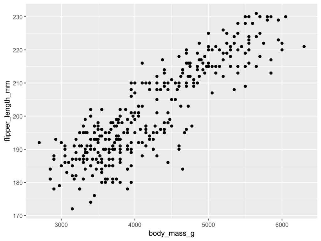
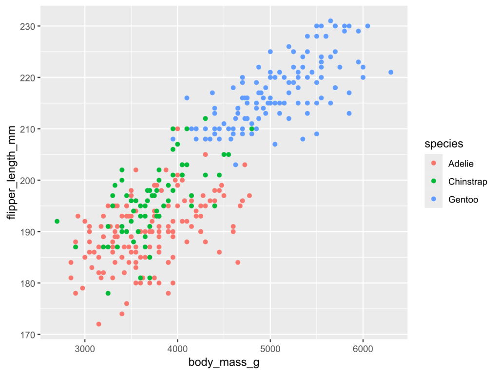
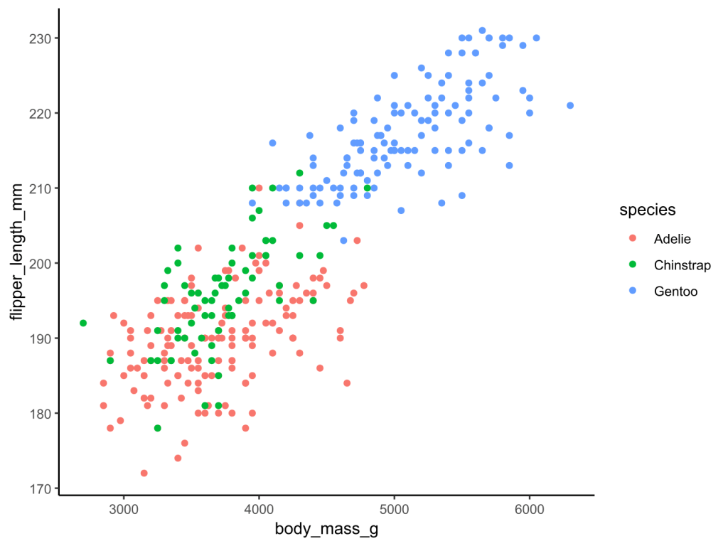
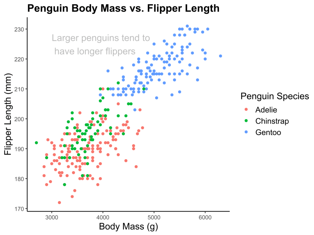
ggplot2 เป็น package สำหรับ data visualisation ในภาษา R และเป็นเครื่องมือสร้างกราฟที่มืออาชีพนิยม ตั้งแต่นักวิจัยในการตีพิมพ์ผลงาน ไปจนถึงสำนักข่าวระดับโลกอย่าง BBC และ Financial Times

ggplot2 มีจุดเด่น 4 ข้อ:

ใช้งานง่าย
สร้างกราฟได้หลากหลาย
ปรับแต่งกราฟได้ดังใจ
ได้กราฟที่ดูดีและมีคุณภาพ

ในบทความนี้ เราจะมาดูวิธีใช้ ggplot2 เพื่อสร้างกราฟแบบมืออาชีพกัน:

ggplot2 syntax
Basic plotting
Plot customisations

ถ้าพร้อมแล้ว ไปเริ่มกันเลย

🔤 gg for “Grammar of Graphics”

gg ใน ggplot2 ย่อมาจาก “Grammar of Graphics”

หนังสือ Grammar of Graphics ของ Leland Wilkinson บน Amazon

Grammar of Graphics เป็นแนวคิดที่มองกราฟเป็นเหมือนภาษา คือ มีโครงสร้างและองค์ประกอบที่ตายตัว ซึ่งเมื่อเรานำมารวมกัน เราก็จะได้กราฟที่ต้องการขึ้นมา

โดยกราฟใน ggplot2 ประกอบด้วย 7 ส่วน หรือ layers ได้แก่:

No.	Layer	Description
1	Data	ชุดข้อมูลสำหรับสร้างกราฟ
2	Aesthetics	จับคู่ข้อมูลกับกราฟ (เช่น แกน x และ y)
3	Geometric objects	ประเภทกราฟ (เช่น กราฟเส้น กราฟแท่ง)
4	Facets	สร้างกราฟย่อย
5	Statistical transformations	วิเคราะห์ข้อมูล (เช่น หาค่าเฉลี่ย)
6	Coordinates	แกนในการสร้างกราฟ
7	Theme	หน้าตาของกราฟ (เช่น สีพื้นหลัง)

ในการทำงาน เรามักจะเรียกใช้งาน 3 layers แรกเป็นหลัก ได้แก่:

Data
Aesthetics
Geometric objects

🏁 Getting Started With ggplot2

ในการเริ่มต้นใช้งาน ggplot2 เราต้องทำ 3 อย่างก่อน คือ:

ข้อที่ 1. ติดตั้ง ggplot2 บน environment ของเรา:

install.packages("ggplot2")

Note: ถ้าใครเคยติดตั้งแล้ว สามารถข้ามไปขั้นถัดไปได้เลย

ข้อที่ 2. เรียกใช้งาน ggplot2:

library(ggplot2)

Note: เราต้องเรียกใช้งาน ggplot2 ทุกครั้งที่เริ่ม session ใหม่

ข้อที่ 3. โหลด dataset ที่เราจะใช้สร้างกราฟ

สำหรับบทความนี้ เราจะใช้ penguins dataset ที่มีข้อมูลของเพนกวิน 3 สายพันธุ์ (เช่น สปีชีส์ น้ำหนัก ความยาวปีก) กัน

เราสามารถโหลด dataset ได้ดังนี้:

install.packages("palmerpenguins")
library(palmerpenguins)

จากนั้น เราสามารถ preview ข้อมูลได้ด้วย head():

head(penguins)

ผลลัพธ์:

Note: เราสามารถอ่านคู่มือ penguins ได้ด้วยคำสั่ง ?penguins

เมื่อทำครบทั้ง 3 ขั้นตอน เราก็พร้อมที่จะสร้างกราฟใน ggplot2 แล้ว

✍️ Basic Syntax

ก่อนไปดูการสร้างกราฟ เรามาดู syntax ของ ggplot2 กันก่อน:

ggplot(data, aes(x, y, other)) +
	geom_*() +
	...

ggplot() คือ การเรียกใช้งาน ggplot2
data คือ ชุดข้อมูลในการสร้างกราฟ
aes() คือ ส่วนจับคู่ข้อมูลกับลักษณะของกราฟ
- x, y คือ ข้อมูลที่แสดงบนแกน x และ y
- other คือ ข้อมูลที่จะแสดงผ่านส่วนอื่น ๆ ของกราฟ เช่น สี ขนาด รูปทรง
geom_* คือ ประเภทกราฟ
… คือ function อื่น ๆ ในการตั้งค่ากราฟ (เช่น theme, facet)

📊 Basic Plotting: Data, Aesthetics, & Geom

ในการสร้างกราฟ เรามี 3 input เบื้องต้นที่เราต้องกำหนด ได้แก่:

No.	Input	Description
1	Data	Dataset ในการสร้างกราฟ
2	Aesthetics	ลักษณะของกราฟที่ใช้แสดงข้อมูล (เช่น แกน x และ y)
3	Geom	ประเภทกราฟ (เช่น กราฟเส้น กราฟแท่ง)

Note: ทั้งสามอย่างสะท้อนถึง 3 layers แรกของ ggplot2

ยกตัวอย่างเช่น

สร้าง scatter plot ที่แสดงความสัมพันธ์ระหว่างน้ำหนักตัว (body_mass_g) และความยาวปีก (flipper_length_mm) ของเพนกวิน:

ggplot(penguins, aes(x = body_mass_g,
                     y = flipper_length_mm)) +
  geom_point()

ผลลัพธ์:

🎨 Aesthetics

นอกจากแกน x และ y เราแสดงข้อมูลผ่านลักษณะอื่น ๆ ของกราฟได้ เช่น:

No.	Parametre	Description
1	`color`	สีขอบรูปทรง
2	`fill`	สีในรูปทรง
3	`shape`	รูปทรง
4	`size`	ขนาด
5	`alpha`	ความโปร่งใส

ยกตัวอย่างเช่น

เพิ่มสปีชีส์เข้าไปใน scatter plot:

ggplot(penguins, aes(x = body_mass_g,
                     y = flipper_length_mm,
                     color = species)) +
  geom_point()

ผลลัพธ์:

Note: เราใช้ color แทน fill เพราะ จุด default ของ scatter plot ไม่รองรับการเติมสี

⏹️ Geom

เราสามารถเปลี่ยนประเภทกราฟได้ โดยเปลี่ยน geom_*() เช่น:

No.	Geom	Graph
1	`geom_histogram()`	Histogram
2	`geom_boxplot()`	Box plot
3	`geom_line()`	Line plot
4	`geom_col()`	Bar plot
5	`geom_density()`	Density plot

Note: ggplot2 มีรูปแบบกราฟกว่า 40+ แบบให้เลือก เราสามารถดูรูปแบบกราฟต่าง ๆ ได้ที่ Function reference และดูตัวอย่างกราฟได้ที่ The R Gallery

นอกจากนี้ เรายังสามารถปรับแต่งหน้าตาของกราฟได้ด้วย parametre ต่าง ๆ ใน geom_*() เช่น:

No.	Parametre	Description
1	`color`	สีขอบรูปทรง
2	`fill`	สีในรูปทรง
3	`shape`	รูปทรง
4	`size`	ขนาด
5	`alpha`	ความโปร่งใส

Note:

จะสังเกตว่า parametre เหล่านี้ (เรียกว่า attribute) เหมือนกับ parametres ของ aes()
ความแตกต่างอยู่ที่ parametre ใน geom_*() จะคงที่ ในขณะที่ parametre ใน aes() จะเปลี่ยนแปลงตามข้อมูล

ยกตัวอย่างเช่น

เปลี่ยนจุดข้อมูลให้เป็นกล่องสี่เหลี่ยมใส:

ggplot(penguins, aes(x = body_mass_g,
                     y = flipper_length_mm,
                     color = species)) +
  geom_point(shape = 22)

ผลลัพธ์:

จะเห็นได้ว่า จุดข้อมูลเปลี่ยนเป็นสี่เหลี่ยมเหมือนกันหมด และไม่เปลี่ยนตามประเภทเพนกวิน เพราะเรากำหนด argument ใน geom_*()

Note: เราสามารถดู argument ของ shape และ parametres อื่น ๆ ได้ที่ Aesthetic specifications

🔧 More Customisations

จนถึงตอนนี้ เรารู้วิธีสร้างและปรับแต่งกราฟเบื้องต้นกันแล้ว

เรามาดู 3 วิธีในการปรับแต่งเพิ่มเติม เพื่อให้กราฟของเราดูเป็นมืออาชีพกัน:

Theme
Text
Facet

🖼️ Theme

Theme ใน ggplot2 หมายถึง หน้าตากราฟที่ไม่เกี่ยวข้องกับข้อมูล เช่น สีแกน x และ y และสีพื้นหลัง

เราสามารถปรับ theme ได้โดยการเรียกใช้ theme_*() เช่น:

ggplot(penguins, aes(x = body_mass_g,
                     y = flipper_length_mm,
                     color = species)) +
  geom_point() +
  
  # Apply classic theme
  theme_classic()

ผลลัพธ์:

จะเห็นว่า กราฟของเราดูสะอาดตามากขึ้น เมื่อไม่มี gridline

Note:

ggplot2 มี built-in themes ให้เลือกใช้ 5 แบบหลัก ได้แก่:

No.	Theme	Background	Gridline
1	`theme_gray()`	สีเทา	สีขาว
2	`theme_classic()`	สีขาว	None
3	`theme_bw()`	สีขาว	สีเทา
4	`theme_light()`	สีขาว	สีเทา
5	`theme_dark()`	สีเทาเข้ม	สีเทาอ่อน

theme_gray() เป็น default theme ของ ggplot2
ดู built-in themes อื่น ๆ ได้ที่ Complete themes
เราสามารถเลือกใช้ themes จาก packages อื่นใน R ได้ เช่น ggthemes และ bbcplot

🔤 Text

ข้อความเป็นส่วนสำคัญของกราฟ ซึ่งสามารถช่วยให้คนที่ดูกราฟของเราเข้าใจกราฟได้ง่ายขึ้น

ใน ggplot2 เราสามารถปรับแต่งข้อความได้ 3 วิธี:

No.	Syntax	Description
1	`theme()`	กำหนดขนาด และ typeface ของข้อความ
2	`labs()`	เพิ่มชื่อกราฟ ชื่อแกน x, y และ legend
3	`annotate()`	เพิ่มโน้ตในกราฟ

ตัวอย่างเช่น:

ggplot(penguins, aes(x = body_mass_g,
                       y = flipper_length_mm,
                       color = species)) +
  geom_point() +
  theme_classic() +
  
  # Adjust text size
  theme(plot.title = element_text(size = 16, face = "bold"),
        axis.title.x = element_text(size = 14),
        axis.title.y = element_text(size = 14),
        legend.title = element_text(size = 14),
        legend.text = element_text(size = 12),
        strip.text = element_text(size = 14, face = "bold")) +
  
  # Add a title, labels, and a legend
  labs(title = "Penguin Body Mass vs. Flipper Length",
       x = "Body Mass (g)",
       y = "Flipper Length (mm)",
       color = "Penguin Species") +
  
  # Add annotation
  annotate("text",
           x = 3000,
           y = 225,
           label = "Larger penguins tend to \\n have longer flippers",
           size = 5,
           color = "gray",
           hjust = 0)

ผลลัพธ์:

จะเห็นได้ว่า กราฟของเรามีชื่อกราฟ คำประกอบแกน x, y และ legend รวมทั้งโน้ตที่ช่วยในการอ่านกราฟ “Larger penguins tend to have longer flippers” เพิ่มขึ้นมา

ในบางครั้ง เราอาจต้องการสร้างกราฟย่อย ซึ่งเราสามารถทำได้ด้วย 2 คำสั่งใน ggplot2:

No.	Function	Dividing Factor
1	`facet_wrap()`	1 categorical variable
2	`facet_grid()`	2 categorical variables

ตัวอย่างเช่น

ใช้ facet_wrap() แบ่งกราฟตามชนิดเพนกวิน:

ggplot(penguins, aes(x = body_mass_g,
                     y = flipper_length_mm,
                     color = species)) +
  geom_point() +
  theme_bw() +
  
  # Use facet_wrap()
  facet_wrap(~species)

ผลลัพธ์:

ใช้ facet_grid() แบ่งตามเพศและชนิดของเพนกวิน:

ggplot(penguins, aes(x = body_mass_g,
                     y = flipper_length_mm,
                     color = species)) +
  geom_point() +
  theme_bw() +
  
  # Use facet_grid()
  facet_grid(sex~species)

ผลลัพธ์:

Note: ในกราฟ เรามี row ที่ 3 (NA) เพราะบาง record ไม่มีข้อมูลเพศของเพนกวิน

🔥 Summary

ในบทความนี้ เราได้เรียนรู้วิธีใช้ ggplot2 เพื่อสร้างกราฟอย่างมืออาชีพ

Syntax ของ ggplot2
การตั้งค่า aesthetics
- x
- y
- Aesthetics อื่น ๆ
การตั้งค่า geom
- geom_*()
- paramatres ของ geom_*()
การปรับแต่งกราฟ
- Theme
- Text
- Facet

📚 Learn More About ggplot2

😺 GitHub

สำหรับผู้ที่สนใจ สามารถดู code ทั้งหมดในบทความนี้ได้ที่ GitHub

📖 Read More About ggplot2

📰 Cheat Sheets

📃 References

Articles:

Courses

✅ R Book for Psychologists: หนังสือภาษา R สำหรับนักจิตวิทยา

📕 ขอฝากหนังสือเล่มแรกในชีวิตด้วยนะครับ 😆

Correlation
t-tests
ANOVA
Reliability
Factor analysis

แล้วทุกคนจะแปลกใจว่า ทำไมภาษา R ง่ายขนาดนี้ 🙂‍↕️

👉 สนใจดูรายละเอียดหนังสือได้ที่ meb:

ดูรายละเอียดหนังสือ R Book for Psychologists

2025-02-20

data.table: แนะนำ 3 ส่วนวิธีใช้งาน package ทรงพลัง เพื่อทำงานกับข้อมูลขนาดใหญ่อย่างมีประสิทธิภาพและรวดเร็ว ในภาษา R แบบครบ — ตัวอย่างการทำงานกับข้อมูลเที่ยวบินจาก flights dataset

R ได้ชื่อว่าเป็น “statistical programming language” เพราะออกแบบมาเพื่อทำงานกับ data โดยเฉพาะ

ภาษา R มี packages มากมายที่รองรับการทำงานกับ data ในรูปแบบตาราง (tabular data) หรือ data frame อย่างตัวอย่างในภาพ:

หนึ่งใน packages ที่ได้รับความนิยมในการทำงานกับ data frame โดยเฉพาะงาน data science ได้แก่ data.table

data.table เป็น package สำหรับ data manipulation ที่มีจุดเด่น 3 อย่าง คือ:

ใช้งานง่าย (แม้จะมีการเขียนที่แตกต่างจาก functions ทั่วไป แต่มี syntax ที่ตายตัว)
ประมวลผลเร็วและประหยัด resource เพราะ data.table optimises code ที่เราเขียน
รองรับการทำงานกับ data ขนาดใหญ่ (เช่น data ที่ใช้ RAM ขนาด 10 ถึง 100 GB ในการประมวลผล)

ในบทความนี้ เราจะมาดูวิธีการใช้งาน data.table แบบครบจบใน 3 ส่วนกัน:

การใช้งาน data.table เบื้องต้น (syntax และ arguments)
การใช้งาน data.table ขั้นสูง (combining และ chaining)
Special symbols ใน data.table

ถ้าพร้อมแล้ว มาเริ่มกันเลย

🏁 Get Started With data.table

ในการเริ่มต้นใช้งาน data.table เราจะต้องทำ 2 อย่าง ได้แก่:

ติดตั้ง data.table (ทำครั้งแรกครั้งเดียว)
โหลด data.table (ทำทุกครั้งที่เริ่ม session ใหม่)

# Install data.table
install.packages("data.table")

# Load data.table
library(data.table)

เมื่อทำทั้ง 2 อย่างนี้แล้ว เราก็พร้อมที่จะใช้งาน data.table กันแล้ว

✈️ Example Dataset: flights

1️⃣ Intro to flights

ในบทความนี้ เราจะมาดูตัวอย่างการใช้ data.table กับ flights ซึ่งมีข้อมูลเที่ยวบินที่ออกจาก New York City ในปี ค.ศ. 2014 เช่น:

วันที่
สนามบินต้นทางและปลายทาง
ระยะเวลาที่เที่ยวบิน delay
ระยะเวลาบิน
ระยะทาง

Note: ดูรายละเอียดทั้งหมดของ dataset ได้ที่ GitHub

2️⃣ Get flights

เราสามารถเริ่มใช้งาน flights ใน 2 ขั้นตอน:

ขั้นที่ 1. Download ไฟล์จาก link โดยไฟล์ที่ได้จะเป็น CSV (comma-separated values):

ขั้นที่ 2. Import ข้อมูลเข้าใน R ด้วย fread() (”fast read”) ซึ่งเป็น function สำหรับโหลดข้อมูลของ data.table:

# Import the dataset
flights <- fread("flights14.csv")

เราสามารถดูตัวอย่างข้อมูลได้ด้วย head():

# Preview the dataset
head(flights)

ผลลัพธ์:

    year month   day dep_delay arr_delay carrier origin   dest air_time distance  hour
   <int> <int> <int>     <int>     <int>  <char> <char> <char>    <int>    <int> <int>
1:  2014     1     1        14        13      AA    JFK    LAX      359     2475     9
2:  2014     1     1        -3        13      AA    JFK    LAX      363     2475    11
3:  2014     1     1         2         9      AA    JFK    LAX      351     2475    19
4:  2014     1     1        -8       -26      AA    LGA    PBI      157     1035     7
5:  2014     1     1         2         1      AA    JFK    LAX      350     2475    13
6:  2014     1     1         4         0      AA    EWR    LAX      339     2454    18

✍️ Syntax: DT[i, j, by]

การใช้งาน data.table ประกอบด้วย 4 ส่วน ดังนี้:

DT[i, j, by]

DT คือ dataset ที่เราต้องการใช้งาน
i ใช้ทำงานกับ rows
j ใช้ทำงานกับ columns
by ใช้จับกลุ่มข้อมูล

เราไปดูรายละเอียดการใช้งาน i, j, และ by กัน

🍦 1st Argument: i

เราสามารถใช้งาน i ได้ 3 อย่าง:

Select rows: เลือก rows ที่ต้องการ
Filter: กรองข้อมูล
Sort: จัดลำดับข้อมูล

1️⃣ Select Rows

เราสามารถใช้ i เพื่อเลือก rows ได้ 3 แบบ:

เลือก 1 row
เลือกหลาย rows
คัด rows ที่ไม่ต้องการออก

แบบที่ #1. เลือก 1 row

เช่น เลือก row ที่ 5 จาก flights:

# Select a row
flights[5]

ผลลัพธ์:

    year month   day dep_delay arr_delay carrier origin   dest air_time distance  hour
   <int> <int> <int>     <int>     <int>  <char> <char> <char>    <int>    <int> <int>
1:  2014     1     1         2         1      AA    JFK    LAX      350     2475    13

แบบที่ #2 – เลือกหลาย rows

ซึ่งเราทำได้โดยการใช้ vector เช่น เลือก rows 1 ถึง 10:

# Select a range of rows
flights[1:10]

ผลลัพธ์:

     year month   day dep_delay arr_delay carrier origin   dest air_time distance  hour
    <int> <int> <int>     <int>     <int>  <char> <char> <char>    <int>    <int> <int>
 1:  2014     1     1        14        13      AA    JFK    LAX      359     2475     9
 2:  2014     1     1        -3        13      AA    JFK    LAX      363     2475    11
 3:  2014     1     1         2         9      AA    JFK    LAX      351     2475    19
 4:  2014     1     1        -8       -26      AA    LGA    PBI      157     1035     7
 5:  2014     1     1         2         1      AA    JFK    LAX      350     2475    13
 6:  2014     1     1         4         0      AA    EWR    LAX      339     2454    18
 7:  2014     1     1        -2       -18      AA    JFK    LAX      338     2475    21
 8:  2014     1     1        -3       -14      AA    JFK    LAX      356     2475    15
 9:  2014     1     1        -1       -17      AA    JFK    MIA      161     1089    15
10:  2014     1     1        -2       -14      AA    JFK    SEA      349     2422    18

หรือเลือก rows 1, 3, 5, 7, และ 9:

# Select multiple rows at interval
flights[c(1, 3, 5, 7, 9)]

ผลลัพธ์:

    year month   day dep_delay arr_delay carrier origin   dest air_time distance  hour
   <int> <int> <int>     <int>     <int>  <char> <char> <char>    <int>    <int> <int>
1:  2014     1     1        14        13      AA    JFK    LAX      359     2475     9
2:  2014     1     1         2         9      AA    JFK    LAX      351     2475    19
3:  2014     1     1         2         1      AA    JFK    LAX      350     2475    13
4:  2014     1     1        -2       -18      AA    JFK    LAX      338     2475    21
5:  2014     1     1        -1       -17      AA    JFK    MIA      161     1089    15

แบบที่ #3 – คัด rows ที่ไม่ต้องการออก

ซึ่งเราสามารถทำได้ 2 แบบ คือ:

ใช้ -
ใช้ !

เช่น คัด row ที่ 1 ออก โดยใช้ -:

# Deselect a row
flights[-1]

หรือใช้ !:

# Deselect a row
flights[!1]

โดยทั้งสองแบบจะให้ผลลัพธ์แบบเดียวกัน แบบนี้:

         year month   day dep_delay arr_delay carrier origin   dest air_time distance  hour
        <int> <int> <int>     <int>     <int>  <char> <char> <char>    <int>    <int> <int>
     1:  2014     1     1        -3        13      AA    JFK    LAX      363     2475    11
     2:  2014     1     1         2         9      AA    JFK    LAX      351     2475    19
     3:  2014     1     1        -8       -26      AA    LGA    PBI      157     1035     7
     4:  2014     1     1         2         1      AA    JFK    LAX      350     2475    13
     5:  2014     1     1         4         0      AA    EWR    LAX      339     2454    18
    ---                                                                                    
253311:  2014    10    31         1       -30      UA    LGA    IAH      201     1416    14
253312:  2014    10    31        -5       -14      UA    EWR    IAH      189     1400     8
253313:  2014    10    31        -8        16      MQ    LGA    RDU       83      431    11
253314:  2014    10    31        -4        15      MQ    LGA    DTW       75      502    11
253315:  2014    10    31        -5         1      MQ    LGA    SDF      110      659     8

2️⃣ Filter

นอกจากการเลือก rows เรายังสามารถใช้ i เพื่อกรอง data ได้ 3 แบบ:

กรองโดยใช้ 1 เงื่อนไข
กรองโดยใช้หลายเงื่อนไข
กรองโดยใช้ helpers

แบบที่ #1 – กรองข้อมูลโดยใช้ 1 เงื่อนไข

เช่น กรอง rows ที่มีระยะทางบิน 500 miles ขึ้นไป:

# Filter with 1 condition
flights[distance >= 500]

ผลลัพธ์:

         year month   day dep_delay arr_delay carrier origin   dest air_time distance  hour
        <int> <int> <int>     <int>     <int>  <char> <char> <char>    <int>    <int> <int>
     1:  2014     1     1        14        13      AA    JFK    LAX      359     2475     9
     2:  2014     1     1        -3        13      AA    JFK    LAX      363     2475    11
     3:  2014     1     1         2         9      AA    JFK    LAX      351     2475    19
     4:  2014     1     1        -8       -26      AA    LGA    PBI      157     1035     7
     5:  2014     1     1         2         1      AA    JFK    LAX      350     2475    13
    ---                                                                                    
198323:  2014    10    31        18       -14      UA    EWR    LAS      291     2227    16
198324:  2014    10    31         1       -30      UA    LGA    IAH      201     1416    14
198325:  2014    10    31        -5       -14      UA    EWR    IAH      189     1400     8
198326:  2014    10    31        -4        15      MQ    LGA    DTW       75      502    11
198327:  2014    10    31        -5         1      MQ    LGA    SDF      110      659     8

แบบที่ #2 – กรองข้อมูลด้วยหลายเงื่อนไข

เราสามารถเพิ่มเงื่อนไขการกรองได้ด้วย logical operators:

Operator	Meaning
`&`	AND
`\|`	OR
`!`	NOT

เช่น กรอง rows ที่:

มีระยะทางบิน 500 miles ขึ้นไป และ
ออกจากสนามบิน LaGuardia (LGA):

# Filter with multiple conditions
flights[distance >= 500 & origin == "LGA"]

ผลลัพธ์:

        year month   day dep_delay arr_delay carrier origin   dest air_time distance  hour
       <int> <int> <int>     <int>     <int>  <char> <char> <char>    <int>    <int> <int>
    1:  2014     1     1        -8       -26      AA    LGA    PBI      157     1035     7
    2:  2014     1     1        -7        -6      AA    LGA    ORD      142      733     5
    3:  2014     1     1        -7         0      AA    LGA    ORD      143      733     6
    4:  2014     1     1        -8       -17      AA    LGA    ORD      139      733     6
    5:  2014     1     1        -2        15      AA    LGA    ORD      145      733     7
   ---                                                                                    
63251:  2014    10    31        14       -17      UA    LGA    IAH      200     1416    17
63252:  2014    10    31        24        -5      UA    LGA    IAH      198     1416     6
63253:  2014    10    31         1       -30      UA    LGA    IAH      201     1416    14
63254:  2014    10    31        -4        15      MQ    LGA    DTW       75      502    11
63255:  2014    10    31        -5         1      MQ    LGA    SDF      110      659     8

แบบที่ #3 – กรองโดยใช้ helpers

เราสามารถกรองข้อมูลโดยใช้ helpers หรือ operators พิเศษ 3 อย่างนี้:

Helper	For	Syntax
`%between%`	กรองข้อมูลตาม range	`col %between% range`
`%like%`	กรองข้อมูลตาม text pattern	`col %like% pattern`
`%chin%`	กรองข้อมูลอยู่ใน set ที่กำหนด	`col %chin% set`

ตัวอย่าง:

ใช้ %between% เพื่อกรองข้อมูลที่มีระยะทางบินระหว่าง 500 ถึง 1,000 miles:

# Filter using %between%
flights[distance %between% c(500, 1000)]

ผลลัพธ์:

        year month   day dep_delay arr_delay carrier origin   dest air_time distance  hour
       <int> <int> <int>     <int>     <int>  <char> <char> <char>    <int>    <int> <int>
    1:  2014     1     1        18        69      AA    JFK    ORD      155      740    17
    2:  2014     1     1        -7        -6      AA    LGA    ORD      142      733     5
    3:  2014     1     1        -7         0      AA    LGA    ORD      143      733     6
    4:  2014     1     1        -8       -17      AA    LGA    ORD      139      733     6
    5:  2014     1     1        -2        15      AA    LGA    ORD      145      733     7
   ---                                                                                    
79754:  2014    10    31        10        -5      UA    EWR    ORD      110      719     6
79755:  2014    10    31         5         2      UA    EWR    ORD      132      719    10
79756:  2014    10    31       427       393      UA    EWR    ORD      100      719    21
79757:  2014    10    31        -4        15      MQ    LGA    DTW       75      502    11
79758:  2014    10    31        -5         1      MQ    LGA    SDF      110      659     8

Note: code นี้ให้ผลลัพธ์เดียวกับการเขียน flights[distance >= 500 & distance <= 1000] แต่การใช้ %between% ทำให้ code สั้นและอ่านง่ายกว่า

ใช้ %like% เพื่อกรองข้อมูลที่สนามบินปลายทางขึ้นต้นด้วย “A” เช่น “ABQ”, “ACK”, “AGS”:

# Filter using %like%
flights[dest %like% "^A"]

ผลลัพธ์:

        year month   day dep_delay arr_delay carrier origin   dest air_time distance  hour
       <int> <int> <int>     <int>     <int>  <char> <char> <char>    <int>    <int> <int>
    1:  2014     1     1        -1         1      AA    JFK    AUS      232     1521    17
    2:  2014     1     1        -5        16      B6    JFK    AUS      247     1521    20
    3:  2014     1     1        21        21      B6    JFK    AUS      237     1521     9
    4:  2014     1     1        10         4      B6    JFK    ABQ      280     1826    20
    5:  2014     1     1        10        10      DL    LGA    ATL      126      762    18
   ---                                                                                    
15630:  2014    10    31        50        43      UA    EWR    ATL      113      746    15
15631:  2014    10    31        -5       -38      UA    EWR    ATL      111      746     5
15632:  2014    10    31        -5        -2      UA    EWR    AUS      211     1504    15
15633:  2014    10    31        -9       -15      UA    EWR    ATL      119      746    11
15634:  2014    10    31        11       -10      UA    EWR    ATL      109      746     8

ใช้ %chin% เพื่อกรองข้อมูลที่สนามบินปลายทาง คือ ATL, LAX, หรือ ORD:

# Filter using %chin%
flights[dest %chin% c("ATL", "LAX", "ORD")]

ผลลัพธ์:

        year month   day dep_delay arr_delay carrier origin   dest air_time distance  hour
       <int> <int> <int>     <int>     <int>  <char> <char> <char>    <int>    <int> <int>
    1:  2014     1     1        14        13      AA    JFK    LAX      359     2475     9
    2:  2014     1     1        -3        13      AA    JFK    LAX      363     2475    11
    3:  2014     1     1         2         9      AA    JFK    LAX      351     2475    19
    4:  2014     1     1         2         1      AA    JFK    LAX      350     2475    13
    5:  2014     1     1         4         0      AA    EWR    LAX      339     2454    18
   ---                                                                                    
38827:  2014    10    31        10        -5      UA    EWR    ORD      110      719     6
38828:  2014    10    31         3       -32      UA    EWR    LAX      320     2454    20
38829:  2014    10    31         5         2      UA    EWR    ORD      132      719    10
38830:  2014    10    31       427       393      UA    EWR    ORD      100      719    21
38831:  2014    10    31        10       -27      UA    EWR    LAX      326     2454    10

3️⃣ Sort

สุดท้าย เราสามารถใช้ i เพื่อเรียงลำดับข้อมูลได้ 3 แบบ:

Sort ascending (A—Z)
Sort descending (Z—A)
Sort by multiple columns

แบบที่ #1 – Sort ascending

เช่น จัดเรียงตามชื่อสนามบินต้นทาง จาก A—Z:

# Sort ascending
flights[order(origin)]

ผลลัพธ์:

         year month   day dep_delay arr_delay carrier origin   dest air_time distance  hour
        <int> <int> <int>     <int>     <int>  <char> <char> <char>    <int>    <int> <int>
     1:  2014     1     1         4         0      AA    EWR    LAX      339     2454    18
     2:  2014     1     1        -5       -17      AA    EWR    MIA      161     1085    16
     3:  2014     1     1       191       185      AA    EWR    DFW      214     1372    16
     4:  2014     1     1        -1        -2      AA    EWR    DFW      214     1372    14
     5:  2014     1     1        -3       -10      AA    EWR    MIA      154     1085     6
    ---                                                                                    
253312:  2014    10    31        24        -5      UA    LGA    IAH      198     1416     6
253313:  2014    10    31         1       -30      UA    LGA    IAH      201     1416    14
253314:  2014    10    31        -8        16      MQ    LGA    RDU       83      431    11
253315:  2014    10    31        -4        15      MQ    LGA    DTW       75      502    11
253316:  2014    10    31        -5         1      MQ    LGA    SDF      110      659     8

แบบที่ #2 – Sorting descending

เราเรียงข้อมูลแบบ descending (Z—A) ได้ 2 วิธี:

ใช้ decreasing = TRUE
ใช้ -

เช่น จัดเรียงตามชื่อสนามบินต้นทาง จาก Z-A โดยใช้ decreasing = TRUE:

# Sort descending with decreasing = TRUE
flights[order(origin, decreasing = TRUE)]

หรือโดยใช้ -:

# Sort descending with -
flights[order(-origin)]

เราจะได้ผลลัพธ์แบบเดียวกัน:

         year month   day dep_delay arr_delay carrier origin   dest air_time distance  hour
        <int> <int> <int>     <int>     <int>  <char> <char> <char>    <int>    <int> <int>
     1:  2014     1     1        -8       -26      AA    LGA    PBI      157     1035     7
     2:  2014     1     1        -7        -6      AA    LGA    ORD      142      733     5
     3:  2014     1     1        -7         0      AA    LGA    ORD      143      733     6
     4:  2014     1     1        -8       -17      AA    LGA    ORD      139      733     6
     5:  2014     1     1        -2        15      AA    LGA    ORD      145      733     7
    ---                                                                                    
253312:  2014    10    31        41        19      UA    EWR    SFO      344     2565    12
253313:  2014    10    31       427       393      UA    EWR    ORD      100      719    21
253314:  2014    10    31        10       -27      UA    EWR    LAX      326     2454    10
253315:  2014    10    31        18       -14      UA    EWR    LAS      291     2227    16
253316:  2014    10    31        -5       -14      UA    EWR    IAH      189     1400     8

แบบที่ #3 – Sort by multiple columns

เช่น จัดเรียงตามชื่อสนามบินต้นทางและปลายทาง ตามลำดับ:

# Sort by multiple columns
flights[order(origin, dest)]

ผลลัพธ์:

         year month   day dep_delay arr_delay carrier origin   dest air_time distance  hour
        <int> <int> <int>     <int>     <int>  <char> <char> <char>    <int>    <int> <int>
     1:  2014     1     2        -2       -25      EV    EWR    ALB       30      143     7
     2:  2014     1     3        88        79      EV    EWR    ALB       29      143    23
     3:  2014     1     4       220       211      EV    EWR    ALB       32      143    15
     4:  2014     1     4        35        19      EV    EWR    ALB       32      143     7
     5:  2014     1     5        47        42      EV    EWR    ALB       26      143     8
    ---                                                                                    
253312:  2014    10    29         0         9      MQ    LGA    XNA      174     1147     6
253313:  2014    10    29        -5       -16      MQ    LGA    XNA      162     1147    14
253314:  2014    10    30        -4       -23      MQ    LGA    XNA      154     1147     6
253315:  2014    10    30        -7       -11      MQ    LGA    XNA      157     1147    14
253316:  2014    10    31        -5       -11      MQ    LGA    XNA      165     1147     6

🧮 2nd Argument: j

เราสามารถใช้ j เพื่อทำงานได้ 3 อย่าง ได้แก่:

Select columns: เลือก columns ที่ต้องการ
Compute: วิเคราะห์ข้อมูล
Create columns: สร้าง columns ใหม่

1️⃣ Select Columns

เราสามารถใช้ j เพื่อเลือก columns ได้ 3 แบบ:

เลือก 1 column
เลือกหลาย columns
คัด columns ที่ไม่ต้องการออก

แบบที่ #1 – เลือก 1 column

เช่น เลือก column สนามบินต้นทาง:

# Select a column
flights[, "origin"]

ผลลัพธ์:

        origin
        <char>
     1:    JFK
     2:    JFK
     3:    JFK
     4:    LGA
     5:    JFK
    ---       
253312:    LGA
253313:    EWR
253314:    LGA
253315:    LGA
253316:    LGA

Note: เราสามารถใช้ตำแหน่ง (1, 2, 3, …) แทนชื่อ columns ("origin") ได้ แต่ไม่เป็นที่นิยม เพราะ columns อาจขยับตำแหน่งได้ และทำให้ผลลัพธ์เปลี่ยนไปได้

แบบที่ #2 – เลือกหลาย columns

เราใช้ j เพื่อเลือกหลาย columns ได้ 3 วิธี:

Vector
List หรือ .()
..

เช่น เลือก 3 columns คือ:

สนามบินต้นทาง
สนามบินปลายทาง
ระยะเวลาบิน

โดยใช้ vector:

# Select multiple columns with a vector
flights[, c("origin", "dest", "air_time")]

ผลลัพธ์:

        origin   dest air_time
        <char> <char>    <int>
     1:    JFK    LAX      359
     2:    JFK    LAX      363
     3:    JFK    LAX      351
     4:    LGA    PBI      157
     5:    JFK    LAX      350
    ---                       
253312:    LGA    IAH      201
253313:    EWR    IAH      189
253314:    LGA    RDU       83
253315:    LGA    DTW       75
253316:    LGA    SDF      110

โดยใช้ list:

# Select multiple columns with a list
flights[, list(origin, dest, air_time)]

หรือใช้ .() ซึ่งเป็น shorthand สำหรับ list:

# Select multiple columns using .()
flights[, .(origin, dest, air_time)]

ผลลัพธ์:

        origin   dest air_time
        <char> <char>    <int>
     1:    JFK    LAX      359
     2:    JFK    LAX      363
     3:    JFK    LAX      351
     4:    LGA    PBI      157
     5:    JFK    LAX      350
    ---                       
253312:    LGA    IAH      201
253313:    EWR    IAH      189
253314:    LGA    RDU       83
253315:    LGA    DTW       75
253316:    LGA    SDF      110

โดยใช้ .. ซึ่งเรามักใช้วิธีนี้เมื่อต้องการเลือก columns แบบ dynamic:

# Select multiple columns using ..

## Create a vector of column names
cols <- c("origin", "dest", "air_time")

## Select using ..
flights[, ..cols]

ผลลัพธ์:

        origin   dest air_time
        <char> <char>    <int>
     1:    JFK    LAX      359
     2:    JFK    LAX      363
     3:    JFK    LAX      351
     4:    LGA    PBI      157
     5:    JFK    LAX      350
    ---                       
253312:    LGA    IAH      201
253313:    EWR    IAH      189
253314:    LGA    RDU       83
253315:    LGA    DTW       75
253316:    LGA    SDF      110

Note: ความแตกต่างระหว่าง vector และ list หรือ .() และ .. คือ:

vector ให้ผลลัพธ์ที่เป็น vector
List หรือ .() และ .. ให้ผลลัพธ์เป็น data.table (data frame ของ data.table)

แบบที่ #3 – คัด columns ที่ไม่ต้องการออก

เราสามารถคัด columns ที่ไม่ต้องการออกได้ 2 วิธี:

ใช้ -
ใช้ !

เช่น เอาชื่อสายการบินออก โดยใช้ -:

# Deselect a column using -
flights[, -c("carrier")]

หรือใช้ !:

# Deselect a column using !
flights[, !c("carrier")]

ผลลัพธ์:

         year month   day dep_delay arr_delay origin   dest air_time distance  hour
        <int> <int> <int>     <int>     <int> <char> <char>    <int>    <int> <int>
     1:  2014     1     1        14        13    JFK    LAX      359     2475     9
     2:  2014     1     1        -3        13    JFK    LAX      363     2475    11
     3:  2014     1     1         2         9    JFK    LAX      351     2475    19
     4:  2014     1     1        -8       -26    LGA    PBI      157     1035     7
     5:  2014     1     1         2         1    JFK    LAX      350     2475    13
    ---                                                                            
253312:  2014    10    31         1       -30    LGA    IAH      201     1416    14
253313:  2014    10    31        -5       -14    EWR    IAH      189     1400     8
253314:  2014    10    31        -8        16    LGA    RDU       83      431    11
253315:  2014    10    31        -4        15    LGA    DTW       75      502    11
253316:  2014    10    31        -5         1    LGA    SDF      110      659     8

2️⃣ Compute

นอกจากการเลือก columns เรายังสามารถใช้ j เพื่อวิเคราะห์หรือข้อมูล (summarise, aggregate) ได้

เช่น หาค่าเฉลี่ยของระยะเวลาบิน:

# Calculate mean
flights[, mean(air_time)]

ผลลัพธ์:

[1] 156.7228

หรือ หาค่าเฉลี่ย และ standard deviation (SD) ของระยะเวลาบิน:

# Calculate mean and SD
flights[, .(avg_air_time = mean(air_time),
            sd_air_time = sd(air_time))]

ผลลัพธ์:

   avg_air_time sd_air_time      n
          <num>       <num>  <int>
1:     156.7228    96.12978 253316

Note: เราสามารถวิเคราะห์ข้อมูลโดยไม่ตั้งชื่อให้กับผลลัพธ์ได้ (avg_air_time, sd_air_time, n) แต่การตั้งชื่อจะช่วยให้เราอ่าน output ได้ง่ายขึ้น

3️⃣ Create Columns

สุดท้าย เราสามารถใช้ j สร้าง columns ใหม่ได้ร่วมกับ:

:= สำหรับสร้าง 1 column
`:=` สำหรับสร้างหลาย columns

เช่น สร้าง column ความเร็วในการบิน (ระยะทาง / เวลา) ด้วย :=:

# Creating 1 new column
flights[, speed := distance / (air_time / 60)]

ผลลัพธ์:

    year month   day dep_delay arr_delay carrier origin   dest air_time distance  hour    speed
   <int> <int> <int>     <int>     <int>  <char> <char> <char>    <int>    <int> <int>    <num>
1:  2014     1     1        14        13      AA    JFK    LAX      359     2475     9 413.6490
2:  2014     1     1        -3        13      AA    JFK    LAX      363     2475    11 409.0909
3:  2014     1     1         2         9      AA    JFK    LAX      351     2475    19 423.0769
4:  2014     1     1        -8       -26      AA    LGA    PBI      157     1035     7 395.5414
5:  2014     1     1         2         1      AA    JFK    LAX      350     2475    13 424.2857
6:  2014     1     1         4         0      AA    EWR    LAX      339     2454    18 434.3363

Note:

เราหาร air_time ด้วย 60 เพื่อแปลงหน่วยจากนาทีเป็นชั่วโมง และทำให้ผลลัพธ์ที่ได้เป็นหน่วย miles/hour
สังเกตว่า column ใหม่จะอยู่ท้ายสุดของ data.table

หรือ สร้าง 2 columns พร้อมกัน เช่น:

ความเร็วในการบิน (ระยะทาง / เวลา)
ระยะเวลาที่ delay โดยรวม (delay ขาออก + delay ขาเข้า)

ด้วย `:=`:

# Creating multiple new column
flights[, `:=`(speed = distance / (air_time / 60),
               total_delay = dep_delay + arr_delay)]

ผลลัพธ์:

    year month   day dep_delay arr_delay carrier origin   dest air_time distance  hour    speed total_delay
   <int> <int> <int>     <int>     <int>  <char> <char> <char>    <int>    <int> <int>    <num>       <int>
1:  2014     1     1        14        13      AA    JFK    LAX      359     2475     9 413.6490          27
2:  2014     1     1        -3        13      AA    JFK    LAX      363     2475    11 409.0909          10
3:  2014     1     1         2         9      AA    JFK    LAX      351     2475    19 423.0769          11
4:  2014     1     1        -8       -26      AA    LGA    PBI      157     1035     7 395.5414         -34
5:  2014     1     1         2         1      AA    JFK    LAX      350     2475    13 424.2857           3
6:  2014     1     1         4         0      AA    EWR    LAX      339     2454    18 434.3363           4

🤝 3rd Argument: by

เราใช้ by เพื่อจับกลุ่มข้อมูล ซึ่งมีประโยชน์มากเวลาที่เราต้องการวิเคราะห์ข้อมูลเป็น ๆ กลุ่ม

เราสามารถใช้ by ได้ 2 แบบ:

จับกลุ่มด้วย 1 column
จับกลุ่มด้วยหลาย columns

แบบที่ #1 – จับกลุ่มด้วย 1 column

เช่น หาค่าเฉลี่ยของ delay ขาออก ตามชื่อสนามบินต้นทาง:

# Group by 1 column
flights[, mean(dep_delay), by = origin]

ผลลัพธ์:

   origin       V1
   <char>    <num>
1:    JFK 11.44617
2:    LGA 10.60500
3:    EWR 15.21248

แบบที่ #2 – จับกลุ่มด้วยหลาย columns

เราจับกลุ่มด้วยหลาย columns ได้ด้วย 2 วิธี คือ:

Vector
List หรือ .()

เช่น หาค่าเฉลี่ยของ delay ขาออก โดยจับกลุ่มตามชื่อสนามบินต้นทางและปลายทาง ตามลำดับ

วิธีที่ 1. ใช้ vector:

# Group by with a vector
flights[, mean(dep_delay), by = c("origin", "dest")]

ผลลัพธ์:

     origin   dest        V1
     <char> <char>     <num>
  1:    JFK    LAX  8.359718
  2:    LGA    PBI 10.168617
  3:    EWR    LAX 15.882631
  4:    JFK    MIA 10.008364
  5:    JFK    SEA 10.858953
 ---                        
217:    LGA    AVL -6.500000
218:    LGA    GSP  6.000000
219:    LGA    SBN  5.000000
220:    EWR    SBN -1.500000
221:    LGA    DAL -6.266667

วิธีที่ 2. ใช้ list:

# Group by with a list
flights[, mean(dep_delay), by = list(origin, dest)]

หรือใช้ .():

# Group by with .()
flights[, mean(dep_delay), by = .(origin, dest)]

ผลลัพธ์:

     origin   dest        V1
     <char> <char>     <num>
  1:    JFK    LAX  8.359718
  2:    LGA    PBI 10.168617
  3:    EWR    LAX 15.882631
  4:    JFK    MIA 10.008364
  5:    JFK    SEA 10.858953
 ---                        
217:    LGA    AVL -6.500000
218:    LGA    GSP  6.000000
219:    LGA    SBN  5.000000
220:    EWR    SBN -1.500000
221:    LGA    DAL -6.266667

Note: เช่นเดียวกับการเลือก columns …

ถ้าเราใช้ vector เราจะได้ผลลัพธ์เป็น vector
ถ้าใช้ list หรือ .() เราจะได้ data.table

🔗 Combining & Chaining

เราสามารถปลอดล็อกพลังที่แท้จริงของ data.table ได้ด้วย 2 วิธี:

Combining: ใช้ i, j, by ร่วมกัน เพื่อตอบโจทย์ที่ซับซ้อน
Chaining: เชื่อมต่อ data.table เข้าด้วยกัน

1️⃣ Combining

ยกตัวอย่างเช่น:

หาค่าเฉลี่ยของความเร็ว
เฉพาะเที่ยวบินที่มีระยะทางตั้งแต่ 500 miles ขึ้นไป
โดยจับกลุ่มตามชื่อสนามบินต้นทาง:

# Combining
flights[distance >= 500, 
        .(avg_speed = mean(distance / (air_time / 60))), 
        by = origin]

อธิบาย code:

distance >= 500 เลือกเฉพาะข้อมูลที่มีระยะทางตั้งแต่ 500 miles ขึ้นไป
.(avg_speed = mean(distance / (air_time / 60))) หาค่าเฉลี่ยของความเร็ว
by = origin] จับกลุ่มข้อมูลด้วยสนามบินต้นทาง

ผลลัพธ์:

   origin avg_speed
   <char>     <num>
1:    JFK  436.6284
2:    LGA  407.5462
3:    EWR  417.1765

2️⃣ Chaining

Chaining คือ การนำ code มาต่อกัน เพื่อส่ง output ต่อกันเป็นทอด ๆ:

DT[...][...][...]

เช่น ค้นหาสนามบินปลายทาง 5 อันดับแรกที่มีค่าเฉลี่ย delay ขาเข้ามากที่สุด ในเดือนสิงหาคม:

# Chaining
flights[month == 8,
        .(avg_arr_delay = mean(arr_delay)),
        by = dest][order(-avg_arr_delay)][1:5]

อธิบาย code:

month == 8 เลือกข้อมูลจากเดือนสิงหาคม
.(avg_arr_delay = mean(arr_delay)) คำนวณค่าเฉลี่ย delay ขาเข้า
by = dest จับกลุ่มตามสนามบินปลายทาง
[order(-avg_arr_delay)] จัดลำดับตามค่าเฉลี่ย delay ขาเข้า แบบ descending
[1:5] เลือกเฉพาะ 5 rows แรกมาแสดง

ผลลัพธ์:

     dest avg_arr_delay
   <char>         <num>
1:    LIT      37.06452
2:    DSM      22.85714
3:    CAK      19.60976
4:    TYS      19.44681
5:    TVC      19.00000

🍩 Special Symbols

เพื่อช่วยให้เราทำงานได้ง่ายขึ้น data.table มี special symbols 3 ตัวที่เราสามารถเรียกใช้ในการทำงานได้:

.N
.SD
.SDcols

1️⃣ .N

.N เป็น special symbol ที่เก็บจำนวน rows ของ data.table เอาไว้ (เช่น 500)

เรามักใช้งาน .N ใน 2 กรณีหลัก ๆ ได้แก่:

เลือก rows
นับจำนวนข้อมูล

กรณีที่ 1. เลือก rows

เช่น เลือก row ที่ 500 จนถึง row สุดท้าย:

# Select rows with .N
flights[500:.N]

ผลลัพธ์:

         year month   day dep_delay arr_delay carrier origin   dest air_time distance  hour
        <int> <int> <int>     <int>     <int>  <char> <char> <char>    <int>    <int> <int>
     1:  2014     1     1        81        86      WN    EWR    HOU      222     1411    17
     2:  2014     1     1        -3        -4      WN    EWR    MDW      128      711     7
     3:  2014     1     1         0        22      WN    EWR    MDW      144      711    12
     4:  2014     1     1        88       190      WN    EWR    MDW      130      711    21
     5:  2014     1     1        45        63      WN    EWR    MDW      141      711    16
    ---                                                                                    
252813:  2014    10    31         1       -30      UA    LGA    IAH      201     1416    14
252814:  2014    10    31        -5       -14      UA    EWR    IAH      189     1400     8
252815:  2014    10    31        -8        16      MQ    LGA    RDU       83      431    11
252816:  2014    10    31        -4        15      MQ    LGA    DTW       75      502    11
252817:  2014    10    31        -5         1      MQ    LGA    SDF      110      659     8

กรณีที่ 2. นับจำนวนข้อมูล

เช่น นับจำนวนข้อมูลการบินตามสนามบินต้นทางแต่ละแห่ง:

# Compute with .N
flights[, .N, by = origin]

ผลลัพธ์:

   origin     N
   <char> <int>
1:    JFK 81483
2:    LGA 84433
3:    EWR 87400

2️⃣ .SD

.SD ย่อมาจาก “Subset of Data” ซึ่งหมายถึง ชุดข้อมูลย่อยที่เกิดจากการจับกลุ่มด้วย by

เรามักใช้ .SD ในการคำนวณคู่กับ lapply() function เพื่อวิเคราะห์ข้อมูลตามกลุ่ม

เช่น หาค่าสูงสุดของแต่ละ columns ในแต่ละเดือน:

# Compute with .SD
flights[,
        lapply(.SD, max, na.rm = TRUE),
        by = month]

ผลลัพธ์:

    month  year   day dep_delay arr_delay carrier origin   dest air_time distance  hour
    <int> <int> <int>     <int>     <int>  <char> <char> <char>    <int>    <int> <int>
 1:     1  2014    31       973       996      WN    LGA    XNA      688     4983    24
 2:     2  2014    28      1014      1007      WN    LGA    XNA      685     4983    24
 3:     3  2014    31       920       925      WN    LGA    XNA      706     4983    24
 4:     4  2014    30      1241      1223      WN    LGA    XNA      664     4983    24
 5:     5  2014    31       889       879      WN    LGA    XNA      650     4983    24
 6:     6  2014    30      1071      1073      WN    LGA    XNA      640     4983    24
 7:     7  2014    31      1087      1090      WN    LGA    XNA      638     4983    24
 8:     8  2014    31       978       964      WN    LGA    XNA      635     4983    24
 9:     9  2014    30      1056      1115      WN    LGA    XNA      635     4983    23
10:    10  2014    31      1498      1494      WN    LGA    XNA      662     4983    24

3️⃣ .SDcols

.SDcols เป็น special symbol ที่เก็บชื่อ columns ของ .SD เอาไว้

เรามักใช้ .SDcols คู่กับ .SD และ lapply() เพื่อวิเคราะห์เฉพาะ columns ที่ต้องการ

เช่น หาเวลา delay สูงสุดของขาเข้าและขาออกในแต่ละเดือน:

# Compute with .SDcols
flights[,
        lapply(.SD, max, na.rm = TRUE),
        by = month,
        .SDcols = c("arr_delay", "dep_delay")]

ผลลัพธ์:

    month arr_delay dep_delay
    <int>     <int>     <int>
 1:     1       996       973
 2:     2      1007      1014
 3:     3       925       920
 4:     4      1223      1241
 5:     5       879       889
 6:     6      1073      1071
 7:     7      1090      1087
 8:     8       964       978
 9:     9      1115      1056
10:    10      1494      1498

😎 Conclusion

ในบทความนี้ เราได้ไปดูวิธีใช้ data.table เพื่อทำทำงานกับข้อมูลขนาดใหญ่กัน

เราได้เห็นว่า data.table มีหลักการเขียนดังนี้:

DT[i, j, by]

และแต่ละ argument มีการใช้งานดังนี้:

Argument i:

Use Case	Example
Select rows	`flights[1:5]`
Filter	`flights[distance >= 500]`
Sort	`flights[order(origin)]`

Argument j:

Use Case	Example
Select columns	`flights[, .(origin, dest)]`
Compute	`flights[, mean(air_time)]`
Create columns	`flights[, speed := distance / (air_time / 60)]`

Argument by:

Use Case	Example
Group data	`flights[by = origin]`

Special symbols:

Symbol	Meaning
`.N`	จำนวน rows
`.SD`	Subset of Data
`.SDcols`	columns ใน Subset of Data

เราสามารถใช้ทุก arguments ร่วมกัน (combining) หรือเชื่อมต่อ data.table (chaining) เพื่อตอบโจทย์ที่ซับซ้อนได้

🎒 Learn More About data.table

😺 GitHub

ดู code ตัวอย่างทั้งหมดในบทความนี้ได้ที่ GitHub

📚 อ่านเพิ่มเติมเกี่ยวกับ data.table

📑 Cheat Sheets ในการใช้งาน data.table

📃 References

✅ R Book for Psychologists: หนังสือภาษา R สำหรับนักจิตวิทยา

📕 ขอฝากหนังสือเล่มแรกในชีวิตด้วยนะครับ 😆

Correlation
t-tests
ANOVA
Reliability
Factor analysis

แล้วทุกคนจะแปลกใจว่า ทำไมภาษา R ง่ายขนาดนี้ 🙂‍↕️

👉 สนใจดูรายละเอียดหนังสือได้ที่ meb:

ดูรายละเอียดหนังสือ R Book for Psychologists

2025-02-13

R Control Flow: วิธีเขียน if, for, while ในภาษา R เพื่อการทำงานที่ง่ายขึ้น พร้อมตัวอย่าง

ในการเขียน code เรามักจะเจอกับงานที่เราต้องทำซ้ำ ๆ เช่น เปลี่ยนตัวเลขในช่วงที่กำหนด (เช่น 80 ถึง 100) ให้เป็นเกรด (เช่น A)

แทนที่เราจะเขียน code ใหม่ทุกครั้งที่เราเจอตัวเลข (เช่น 89, 82, 91) เราสามารถใช้ control flow เข้ามาช่วย automate งาน ลดเวลาและภาระงานของเราลงไปได้

ในบทความนี้ เราจะมาดูวิธีเขียน control flow ในภาษา R กัน:

If-else:
- if
- else
- else if
Loops:
- for
- while
Loop control:
- next
- break

ถ้าพร้อมแล้ว มาเริ่มกันเลย

🕹️ If-Else

ในการเขียน if-else เรามี 3 syntax ที่ต้องทำความเข้าใจ:

if
else
else if

1️⃣ if

เราใช้ if เพื่อกำหนดเงื่อนไขในการทำงาน

เช่น ถ้าคะแนนมากกว่า 60 ให้ผ่าน:

if (score >= 60) {
	print("Pass")
}

ถ้าไม่ตรงกับเงื่อนไข R จะรัน code บรรทัดถัดไป

2️⃣ else

เราใช้ else เพื่อกำหนด action ที่ต้องทำเมื่อข้อมูลไม่เข้าเงื่อนไข

เช่น ถ้าน้อยกว่า 60 ให้ไม่ผ่าน:

if (score >= 60) {
	print("Pass")
} else {
	print("Fail")
}

ในครั้งนี้ R จะแสดงคำว่า “Pass” หรือ “Fail” ก่อนจะรัน code บรรทัดถัดไป

3️⃣ else if

ถ้าเรามีมากกว่า 2 เงื่อนไข ให้ใช้ else if เพื่อกำหนดเงื่อนไขเพิ่มเติม

เช่น ตัดเกรดตามช่วงคะแนน:

if (score >= 90) {
	print("A")
} else if (score >= 80) {
	print("B")
} else if (score >= 70) {
	print("C")
} else if (score >= 60) {
	print("D")
} else {
	print("F")
}

ใน code นี้ R จะรันแต่ละบรรทัด และถ้าข้อมูลที่มีตรงกับเงื่อนไข ก็จะทำตาม action ในบรรทัดนั้น

เช่น เรากำหนดให้:

score <- 71

R จะรัน else if จนถึงบรรทัดที่ 5 แล้วทำ action ที่อยู่ในบรรทัด 6:

🔁 Loops

Loops ใช้ในการทำ task ซ้ำเรื่อย ๆ ตามเงื่อนไขที่กำหนด

เราสามารถเขียน loop ได้ 2 แบบ คือ:

for
while

1️⃣ for

for ใช้สำหรับทำงานซ้ำ ๆ ที่เรารู้ว่าจะต้องทำกี่ครั้ง

เช่น เรามีรายชื่อเพื่อนที่เราอยากจะทักทาย:

friends <- c("John",
             "Sarah", 
             "Emma",
             "Mike")

เราสามารถใช้ for loop ช่วยได้แบบนี้:

for (friend in friends) {
  print(paste("Hello,", friend))
}

ผลลัพธ์:

2️⃣ while

เราใช้ while เมื่อต้องทำงานซ้ำ ๆ ที่เราไม่รู้ว่าจะต้องทำกี่ครั้ง

โดย while จะทำงานไปเรื่อย ๆ จนกว่าเงื่อนไขที่กำหนดจะไม่เป็นจริง

เช่น ทอยเต๋าเรื่อย ๆ จนกว่าจะได้เลข 6:

set.seed(42)

roll <- sample(1:6, 1)

while (roll != 6) {
  print(paste("Rolled:", roll, "Not yet..."))
  roll <- sample(1:6, 1)
}

print("You rolled a 6! Congratulations!")

อธิบาย code:

Code	Explain
`set.seed(42)`	ทำให้ code ให้ผลลัพธ์เหมือนกันทุกครั้ง
`sample(1:6, 1)`	สุ่ม 1 เลข ระหว่าง 1 ถึง 6
`while (roll != 6) {...}`	จนกว่า roll จะเท่ากับ 6 ให้ทำ action ใน `{...}`
`print("You rolled a 6! Congratulations!")`	ถ้าหลุดจาก while loop แล้ว ให้ print “You rolled a 6! Congratulations!”

ถ้ารัน code แล้ว เราจะได้ผลลัพธ์แบบนี้:

จะเห็นว่า while loop หยุดเมื่อ roll != 6 ไม่เป็นจริง (เมื่อ roll = 6)

🚸 Loop Control

ในการเขียน for และ while loops เรามี 2 statements ที่ช่วยกำกับ loops ได้ คือ:

next
break

1️⃣ next

next ใช้เพื่อข้ามข้อมูลที่เราไม่ต้องการให้เกิด action

เช่น เรามี list ของสี:

colours <- c("🟢", "🔴", "🔵", "🔴", "🟠", "🟢")

ซึ่งเราต้องการ print เฉพาะสีโทนเย็น (skip สีโทนร้อน เช่น 🔴, 🟠) เราสามารถใช้ next คู่กับ if และ for ได้แบบนี้:

for (colour in colours) {
  if (colour == "🔴" | colour == "🟠") next
  print(colour)  
}

ผลลัพธ์:

จะเห็นได้ว่า code ของเราข้ามข้อมูลที่เป็นสีโทนร้อน และ print เฉพาะสีโทนเย็นออกมา

2️⃣ break

break ทำหน้าที่คล้าย next

แต่แทนที่จะข้ามข้อมูลไป break จะหยุดการทำงานของ loop และปล่อยให้ R รัน code บรรทัดหลังจาก loop ได้

เช่น เรามี while loop ที่นับเลขตั้งแต่ 10 ถึง 0:

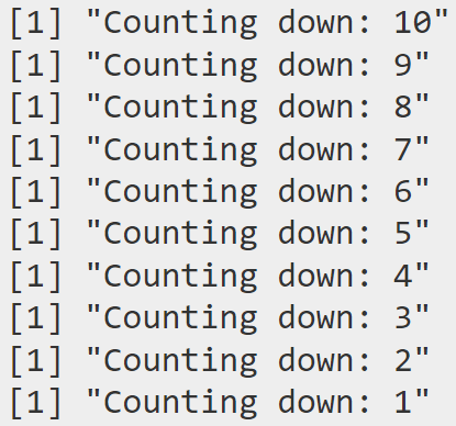
time <- 10  # Start countdown

while (time > 0) {
  print(paste("Counting down:", time))
  time <- time - 1
}

ถ้าเราไม่ใส่ break, while loop ของเราจะนับเลขถึง 0:

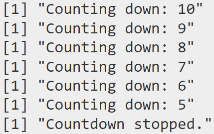
แต่ถ้าเราใส่ break เข้าไป while loop จะหยุดนับ ณ ตัวเลขที่เรากำหนด:

time <- 10  # Start countdown

while (time > 0) {
  if (time == 4) {
    print("Countdown stopped.")
    break  # Stop the loop when time reaches 4
  }
  print(paste("Counting down:", time))
  time <- time - 1
}

ผลลัพธ์:

จะเห็นได้ว่า break ทำให้ while loop หยุดทำงาน เมื่อนับถึง 4

💪 Summary

ในบทความนี้ เราเรียนรู้วิธีเขียน control flow ใน R กัน:

If-else:

Statement	Description
`if`	กำหนด 1 เงื่อนไข
`else`	ทำ action เมื่ออยู่นอกเงื่อนไข
`else if`	เพิ่มเงื่อนไข

Loops:

Statement	Description
`for`	repeat task เมื่อรู้ว่า action ที่ต้องทำจะเกิดขึ้นกี่ครั้ง
`while`	repeat task เมื่อไม่รู้ว่า action ที่ต้องทำจะเกิดขึ้นกี่ครั้ง

Loop control:

Statement	Description
`next`	Skip ข้อมูลใน loop
`break`	หยุด loop

🗒️ Practice Control Flow

แม้ว่าตัวอย่างในบทความนี้จะเป็นตัวอย่างง่าย ๆ แต่ control flow เป็นการเขียน code ที่มีประโยชน์มาก และสามารถใช้แก้ปัญหาทั้งเล็กและใหญ่ในโลกจริงได้ เช่น:

ส่ง update ข้อมูล PM2.5 รายวัน
เช็ก username และ password เพื่อยืนยันการเข้าสู่ระบบ
ทำระบบสั่งอาหารและจ่ายเงินออนไลน์
สร้างเกมเป่ายิ้งฉุบ
สร้างระบบกดเงิน ATM

และอีกมากมาย

สำหรับคนที่สนใจสามารถลองเขียน control flow เพื่อแก้ปัญหาเหล่านี้ได้

ติดตั้ง R และ RStudio เพื่อใช้งาน R:

Install R: https://cran.r-project.org/bin/windows/base/
Install RStudio: https://posit.co/download/rstudio-desktop/
ใช้ RStudio แบบออนไลน์: https://posit.cloud/

😺 GitHub

ดูตัวอย่าง code ในบทความนี้ได้ที่ GitHub

📃 References

✅ R Book for Psychologists: หนังสือภาษา R สำหรับนักจิตวิทยา

📕 ขอฝากหนังสือเล่มแรกในชีวิตด้วยนะครับ 😆

Correlation
t-tests
ANOVA
Reliability
Factor analysis

แล้วทุกคนจะแปลกใจว่า ทำไมภาษา R ง่ายขนาดนี้ 🙂‍↕️

👉 สนใจดูรายละเอียดหนังสือได้ที่ meb:

ดูรายละเอียดหนังสือ R Book for Psychologists

2025-02-06

R Foundation: ทำความรู้จักกับภาษา R สำหรับผู้เริ่มต้น – ภาษา R คืออะไร, ต่างกับ Python ยังไง, และเขียนยังไง?

ในบทความนี้ เราจะมาทำความรู้จักภาษา R กัน:

ภาษา R คืออะไร?
R แตกต่างกับ Python ยังไง?
พื้นฐานการเขียนภาษา R

ถ้าพร้อมแล้วมาเริ่มกันเลย

ภาษา R คืออะไร?

R เป็นภาษาคอมพิวเตอร์ที่ถูกพัฒนาขึ้นในช่วง ค.ศ. 1990 โดยนักสถิติ 2 ท่านจาก University of Auckland ในนิวซีแลนด์:

Ross Ihaka
Robert Gentleman

โดยทั้งคู่พัฒนา R เพื่อทำงานกับข้อมูลในห้องแล็บโดยเฉพาะ

และด้วยเหตุที่ R ถูกออกแบบมาเพื่อทำงานกับข้อมูล จึงได้ชื่อว่าเป็น “statistical programming language”

Note: ตัวอักษรแรกของนักพัฒนาเป็นที่มาของชื่อภาษา

“Logo for R” by The R Foundation (from https://www.r-project.org/logo/ under the CC-BY-SA 4.0)

เพราะ R เป็นภาษาสำหรับ data จึงเป็นที่นิยมในสายอาชีพ data อย่าง:

Data analyst
Data scientist
Business intelligence analyst
Statistician
Researcher

ในปัจจุบัน (Jan 2025) R ได้รับความนิยมเป็นอันดับ 18 ของโลก (อ้างอิง TIOBE index):

นอกจากเป็นภาษา data แล้ว R ยังได้รับความนิยม เพราะ:

เป็นภาษา open source
ผู้ใช้งานสามารถสร้าง package (library) ในการวิเคราะห์ข้อมูลเองได้
ผู้ใช้สามารถใช้ package ที่คนอื่นเขียนไว้แล้ว มาวิเคราะห์ข้อมูลได้ (ในปัจจุบัย R มี package ให้เลือกใช้งานมากกว่า 17,000 packages)
ใช้งานได้กับหลากหลาย OS เช่น Windows, MacOS, และ Linux

R vs Python: แตกต่างกันยังไง?

ทั้ง R และ Python ต่างได้เป็นที่นิยมในสายงาน data science และมีลักษณะที่คล้ายกัน คือ:

เป็นภาษา open source
มี community ผู้ใช้งานขนาดใหญ่
มี packages ให้เลือกใช้จำนวนมาก

แต่ R และ Python จุดที่แตกต่างกัน คือ:

R	Python
เหมาะกับการทำงาน data โดยเฉพาะการวิเคราะห์สถิติเชิงลึก	เป็นภาษาสำหรับงานทั่วไป (general-purpose) รองรับการใช้งานหลายประเภทกว่า R

ดังนั้น แม้ว่า R อาจจะสามารถทำงานนอกเหนือจากงาน data ได้ (เช่น web scrapping) แต่อาจจะไม่ดีเท่ากับ Python ที่ถูกออกแบบมาให้ใช้งานทั่วไป

Note:

สำหรับคนที่สนใจสายงาน data ควรเลือกศึกษาทั้ง 2 ภาษา

แต่การจะหยิบมาใช้งาน ขึ้นอยู่กับงานตรงหน้า:

R	Python
งานวิจัยและการวิเคราะห์ข้อมูลเชิงลึก เช่น สร้างโมเดลทางสถิติ รวมทั้งการสร้างกราฟจากข้อมูลอย่างง่าย	งานที่ต้องมีความยืดหยุ่น เช่น machine learning และ AI หรืองานที่ต้อง integrate กับเครื่องมืออื่น ๆ เช่น web scrapping และ software development

Objects & Functions: โลกทั้งใบของ R

หลังจากทำความรู้จักความรู้จักกับ R เบื้องต้นแล้ว เรามาดูหลักการทำงานของ R กัน

ในการทำงานกับ R เราต้องเข้าใจก่อนว่า ทุกสิ่งที่อยู่ใน R ประกอบด้วย 2 อย่าง ได้แก่:

Object	Function
สิ่งที่เก็บใน R	สิ่งที่เกิดขึ้นใน R

นั่นคือ:

ทุกสิ่งที่เราสร้างขึ้นใน R จะถูกเก็บอยู่ใน objects (เช่น ตัวแปร, ข้อมูล)
Functions เป็นสิ่งที่เรากระทำกับ objects (เช่น การคำนวณ การสร้างกราฟ)

เมื่อเราเข้าใจแล้ว เราสามารถทำความเข้าใจ concepts อื่น ๆ ของ โดยการต่อยอดจาก 2 องค์ประกอบนี้

Objects: Existing in R

ในส่วน objects เรามี 3 สิ่งที่ต้องความเข้าใจ เพื่อทำงานกับ R:

Variables
Data types and classes
Data structures

📦 (1) Variables: การประกาศตัวแปรใน R

Variable หรือตัวแปร เป็นเหมือนกล่องเก็บของที่เก็บข้อมูลไว้ให้เรา

เราสามารถสร้างตัวแปรด้วยการใช้ <- เช่น:

x <- 10

อย่างในตัวอย่าง เป็นการสร้างตัวแปร x ที่เก็บค่าตัวเลข 10 เอาไว้

Note: เราสามารถใช้ = แทน <- ได้ แต่ไม่เป็นที่นิยมกัน

🍱 (2) Data Types & Classes: ประเภทข้อมูลใน R

ตัวแปรใน R สามารถเก็บข้อมูลได้หลายประเภท (เช่น ตัวเลข ข้อความ)

เราต้องทำความเข้าใจประเภทของข้อมูล เพราะเป็นตัวกำหนด functions ที่เราสามารถใช้ทำงานกับ variable นั้นได้

ยกตัวอย่างเช่น x เก็บตัวแปรประเภทตัวเลข เราจะไม่สามารถใช้ functions ที่ทำงานกับตัวอักษรได้

ทั้งนี้ ประเภทข้อมูลใน R มีอยู่ 5 ประเภทที่มักใช้บ่อย ได้แก่:

No.	Data Type	Example
1	Numeric	`100`
2	Character	`"One hundred"`
3	Logical	`TRUE`, `FALSE`
4	Date	`2025-01-15`
5	Factor	`"male"`, `"female"`, `"other"`

ตัวอย่าง 👇

Numeric:

age <- 10

Character:

name <- "Ben Tennyson"

Logical:

is_hero <- TRUE

Date:

date_of_birth <- as.Date("1995-12-27")

Factor:

gender <- as.factor("Male")

Note: เราสามารถเช็กประเภทข้อมูลของตัวแปร ได้ด้วย class() เช่น:

class(age)

ผลลัพธ์:

🏠 (3) Data Structures: โครงสร้างข้อมูลใน R

Data structure เป็นการนำข้อมูลมาจัดเรียงเป็นโครงสร้างที่ใหญ่ขึ้น

Data structures เป็นเหมือนอิฐที่ประกอบกันเป็นบ้านหรือตึกใน R

โครงสร้างข้อมูลใน R มีอยู่ 5 ประเภท ซึ่งแบ่งได้เป็น 2 กลุ่มตามมิติในการเก็บข้อมูล ดังนี้:

กลุ่มที่ 1: เก็บข้อมูลได้ 1 ประเภทเท่านั้น

No.	Data Structure	การเก็บข้อมูล
1	Vector	1 มิติ
2	Matrix	2 มิติ
3	Array	n มิติ

ตัวอย่าง 👇

Vector:

v <- c(1, 3, 5, 7, 9)

ผลลัพธ์:

Matrix:

m <- matrix(1:9, ncol = 3)

ผลลัพธ์:

Array:

เช่น array แบบ 3 มิติ:

4 rows
3 columns
2 ชั้น

a <- array(1:24, dim = c(4, 3, 2))

ผลลัพธ์:

กลุ่มที่ 2: เก็บข้อมูลได้มากกว่า 1 ประเภท

No.	Data Structure	การเก็บข้อมูล
1	List	1 มิติ
2	Data frame	2 มิติ

ตัวอย่าง 👇

List:

เพราะ list สามารถเก็บข้อมูลได้หลายประเภท เราสามารถใส่อะไรลงใน list ก็ได้ (แม้แต่ data structure อื่น ๆ):

grocery_list = list("apple",
                    "milk",
                    TRUE,
                    250,
                    c(1, 3, 5, 7, 9),
                    list("Walmart", "Target"))

ผลลัพธ์:

Data frame:

สำหรับ data frame เราสามารถสร้างได้จากเชื่อม vectors เข้าด้วยกัน:

groceries <- data.frame(
  Item = c("Apples", "Carrots", "Milk"),
  Category = c("Fruit", "Vegetable", "Dairy"),
  Quantity = c(5, 2, 1),
  Price = c(1.50, 0.75, 2.50)
)

ผลลัพธ์:

Note: สำหรับใครที่นึกภาพโครงสร้างข้อมูลไม่ออก สามารถดู Figure 5.6 ในหนังสือ Hands-On R Programming เพื่อช่วยไขข้อสงสัยได้

Functions: Happening in R

สำหรับ functions เรามี 2 สิ่งที่ต้องทำความเข้าใจ ได้แก่:

Operators
Functions

🧮 (1) Operators: เครื่องหมายใน R

Operators เป็นเครื่องหมาย เพื่อบอก R ว่าเราต้องการทำงานหรือการคำนวณอะไร

Operators แบ่งออกเป็น 4 ประเภท ได้แก่:

No.	Operator	For	Symbols
1	Assignment	สร้าง variable	`<-` `=`
2	Arithmetic	คิดเลข	`+` `-` `*` `/`
3	Logical	คิดตรรกะ	`&` `\|` `!`
4	Relational	เปรียบเทียบค่า	`==` `!=` `>` `<` `>=` `<=`

ตัวอย่าง 👇

Assignment

เช่น สร้างตัวแปรเก็บชื่อ “John”:

my_name <- "John"

Arithmetic

เช่น คิดเลข 3 + 4:

3 + 4

Logical

เช่น not TRUE:

!TRUE

Relational

เช่น เช็กว่า 15 มากกว่า 11 ไหม:

15 > 11

🔨 (2) Functions: Action ใน R

Functions คือ code ที่เราสามารถนำกลับมาใช้ใหม่ได้ (reusable)

Functions แบ่งออกเป็น 2 ประเภท ได้แก่:

No.	Function	Description	Example
1	Built-in	Functions ที่มาพร้อม R หรือ packages ที่เราโหลดมาใช้งาน	`print()` `sum()` `str()`
2	User-defined	Functions ที่เราสร้างเอง	สร้าง function ชื่อ `hello()` เพื่อทักทาย user

Note:

สำหรับ user-defined functions เราสามารถสร้างได้โดยใช้ function() เช่น:

greeting <- function(name) {
  print(paste("Hello", name))
}

ถ้าเราเรียกใช้งาน greeting() โดยใส่ "John" ใน ():

greeting("John")

เราจะได้ผลลัพธ์แบบนี้:

Conclusion

ในบทความนี้ เราได้ทำความรู้กับภาษา R กัน:

R เป็นภาษาสำหรับงาน data
ทั้ง R และ Python ใช้กับงาน data ได้
- R เหมาะกับการวิเคราะห์เชิงลึก
- Python เหมาะกับงานทั่วไป
- คนที่สนใจงานสาย data ควรเรียนทั้ง 2 ภาษา
ทุกอย่างใน R แบ่งเป็น objects และ functions
Objects: สิ่งที่เก็บใน R
- Variables: เก็บข้อมูล
- Data types and classes: กำหนด functions
- Data structures: ประกอบร่างข้อมูล
Functions: สิ่งที่เกิดขึ้นใน R
- Operators: เครื่องหมายในการทำงาน
- Functions: code ที่นำกลับมาใช้ใหม่ได้

Learn More About R

🧑‍💻 GitHub

สำหรับผู้ที่สนใจ สามารถดู code ตัวอย่างในบทความนี้ได้ที่ GitHub

🔨 Free Tool

เริ่มทดลองเขียน R ด้วยตัวเอง ผ่าน RStudio

ติดตั้งและใช้งานบน desktop : https://posit.co/downloads/
ใช้งาน online: https://posit.cloud/

ดาวน์โหลด R

Windows: https://cran.r-project.org/bin/windows/base/
macOS: https://cran.r-project.org/bin/macosx/

Note: ใช้งานฟรีทั้งแบบ desktop และ online

📗 Free e-Books

ใครที่สนใจเรียนรู้เกี่ยวกับ R เพิ่มเติม สามารถอ่านหนังสือ e-book เหล่านี้ได้ฟรี:

🏫 Free Courses

สำหรับคนที่สนใจเรียนการเขียน R สามารถศึกษาคอร์สเรียนเหล่านี้ได้:

R Crash Course จาก DataRockie
HarvardX: Data Science: R Basics จาก edX

References

✅ R Book for Psychologists: หนังสือภาษา R สำหรับนักจิตวิทยา

📕 ขอฝากหนังสือเล่มแรกในชีวิตด้วยนะครับ 😆

Correlation
t-tests
ANOVA
Reliability
Factor analysis

แล้วทุกคนจะแปลกใจว่า ทำไมภาษา R ง่ายขนาดนี้ 🙂‍↕️

👉 สนใจดูรายละเอียดหนังสือได้ที่ meb:

ดูรายละเอียดหนังสือ R Book for Psychologists

2025-01-30

เล่นกับข้อมูลง่าย ๆ ด้วย 5 functions จาก dplyr: วิธีใช้งาน dplyr เบื้องต้น พร้อมตัวอย่างการทำงานกับข้อมูล HR

💻 ภาษา R

R เป็นภาษาคอมพิวเตอร์ที่ออกแบบมาเพื่อทำงานกับ data เหมาะกับสายงานที่ต้องทำงานกับ data เช่น

Researcher ที่ต้องการวิเคราะห์ลักษณะกลุ่มตัวอย่าง เช่น จำนวนตัวอย่างแบ่งตามเพศ หรือช่วงอายุ
Data analyst ที่ต้องการหา insight จากข้อมูลขององค์กร เช่น วิเคราะห์แนวโน้มทางธุรกิจ
Sale ที่ต้องการวิเคราะห์ข้อมูลการขาย เช่น จำนวนลูกค้า ยอดขาย และกำไร
หรือแม้แต่ HR ที่ต้องการทำข้อมูลพนักงาน เช่น วิเคราะห์ performance, engagement, และ job satisfaction

🔢 dplyr: Library สำหรับหมุนข้อมูล

R มี built-in functions และ libraries หลากหลายที่รองรับการทำงานกับ data ในรูปแบบต่าง ๆ ซึ่งหนึ่งใน libraries ที่นิยมใช้กัน ได้แก่ dplyr

dplyr เป็น library ที่ออกแบบมาเพื่อ data transformation หรือการแปลงข้อมูล ช่วยให้การทำงานกับ data ง่ายขึ้น เมื่อเทียบกับ built-in functions

Use case ของ dplyr เช่น:

สำรวจข้อมูล (data exploration)
ทำความสะอาดข้อมูล (data cleaning)
วิเคราะห์ข้อมูล (data analysis)

ในบทความนี้ เราจะไปทำความรู้จักกับ 5 functions พื้นฐานของ dplyr ที่ใช้ทำงานกับข้อมูลกัน ซึ่งได้แก่:

select()
filter()
arrange()
summarise() หรือ summarize() (เขียนได้ทั้งสองแบบ)
mutate()

🧑‍💼 ตัวอย่างข้อมูล HR

ในบทความนี้ เราจะใช้ชุดข้อมูลจำลอง hr_data เพื่อช่วยอธิบายการใช้งาน 5 functions ของ dplyr

hr_data ช่วยจำลองสถานการณ์ของ HR ที่ต้องวิเคราะห์ข้อมูลพนักงาน เพื่อหาวิธีแก้ปัญหาพนักงานลาออก (attrition)

โดย hr_data ประกอบด้วย 8 ตัวแปร:

No.	Column	Data
1	`ID`	รหัสพนักงาน
2	`Name`	ชื่อพนักงาน
3	`Department`	แผนก
4	`Age`	อายุ
5	`Engagement`	คะแนนการมีส่วนร่วม (1 ถึง 100)
6	`YearsAtCompany`	อายุงาน
7	`AttritionRisk`	ความเสี่ยงที่จะลาออก (Low, Medium, High)
8	`Salary`	เงินเดือน

Code ในการสร้างและเรียกดู hr_data:

# Create the dataset
hr_data <- data.frame(
  ID = 1:15,
  Name = c("Alice", "Bob", "Carol", "David", "Eve", "Frank", "Grace", 
           "Henry", "Ivy", "Jack", "Karen", "Liam", "Mona", "Nate", "Olivia"),
  Department = c("HR", "IT", "Finance", "HR", "Sales", "IT", "Finance", 
                 "Sales", "IT", "HR", "Finance", "Sales", "IT", "HR", "Sales"),
  Age = c(34, 29, 45, 50, 27, 30, 42, 35, 31, 40, 38, 28, 33, 55, 26),
  Engagement = c(85, 70, 65, 55, 90, 75, 60, 88, 80, 50, 68, 72, 78, 40, 95),
  YearsAtCompany = c(5, 2, 15, 25, 1, 3, 10, 7, 4, 20, 12, 1, 6, 30, 0),
  AttritionRisk = c("Low", "Medium", "High", "High", "Low", "Medium", "High", 
                    "Low", "Medium", "High", "High", "Low", "Medium", "High", "Low"),
  Salary = c(55000, 60000, 70000, 75000, 50000, 62000, 68000, 58000, 
             61000, 77000, 72000, 51000, 64000, 80000, 49000)
)

# View the dataset
hr_data

ผลลัพธ์:

✍️ Pattern การเขียน Function

แม้ว่าทั้ง 5 functions จะมีหน้าที่แตกต่างกัน แต่มีการเรียกใช้งานที่เหมือนกัน:

func(dataset,
     condition)

func = ชื่อ function เช่น select, filter, arrange
dataset = ชุดข้อมูลที่เป็น input
condition = เงื่อนไขในการใช้งานทำงานของ function

1️⃣ Function #1: select()

select() ใช้เลือก column ข้อมูลที่ต้องการ

ตัวอย่าง:

ผู้บริหารต้องการข้อมูลที่มีแค่รายชื่อพนักงาน แผนก และคะแนนการมีส่วนร่วม

เราสามารถใช้ select() เลือกเฉพาะ column ที่ต้องการได้:

# Select only desired columns
select(hr_data,
       Name,
       Department,
       Engagement)

ผลลัพธ์:

Note:

เวลาเลือก column ด้วย select() เราสามารถกำหนดลำดับของ column ที่จะมาแสดงได้ เช่น ต้องการแสดง Department ก่อน Name ก็ให้เขียน Department, Name

dplyr มี helper function ที่ช่วยในการเลือก column ให้ง่ายขึ้น เช่น:

Function	Meaning
`starts_with()`	เลือก column ที่เริ่มด้วย x
`ends_with()`	เลือก column ที่ลงท้ายด้วย x
`contains()`	เลือก column ที่มีคำว่า x
`matches()`	เลือก column ที่ตรงกับ regular expression
`last_col()`	เลือก column สุดท้ายในชุดข้อมูล
`~`	เลือกทุก column ยกเว้น column ที่ระบุ

เราสามารถตั้งชื่อ column ใหม่ได้ ด้วยใช้ = เช่น FullName = Name เพื่อให้หัว column แสดงคำว่า Fullname แทน Name

2️⃣ Function #2: filter()

filter() ใช้เลือก row ที่ตรงกับเงื่อนไขที่กำหนดมาแสดง

ตัวอย่าง:

ผู้บริหารต้องการข้อมูลพนักงานที่ความเสี่ยงที่จะลาออกสูง

เราสามารถใช้ filter() เพื่อกำหนดเงื่อนไขเพื่อกรองข้อมูลออกมาได้:

# Filter for high attrition risk
filter(hr_data,
       AttritionRisk == "High")

ผลลัพธ์:

Note:

เราสามารถใช้ boolean operator และ comparison operator ร่วมได้:

Operator	Meaning
`==`	เท่ากับ
`!=`	ไม่เท่ากับ
`>`	มากกว่า
`<`	น้อยกว่า
`&`	and
`\|`	or
`!`	not

เช่น:

ผู้บริหารต้องการข้อมูลพนักงานที่ความเสี่ยงที่จะลาออกสูง ในแผนกการเงิน (Finance)

# Filter for high attrition risk in Finance
filter(hr_data,
       AttritionRisk == "High" & Department == "Finance")

ผลลัพธ์:

3️⃣ Function #3: arrange()

arrange() ใช้เรียงข้อมูลตามเงื่อนไข

ตัวอย่าง:

ผู้บริหารอยากได้ข้อมูลพนักงานเรียงจากคะแนนการมีส่วนร่วม

เราสามารถใช้ arrange() จัดลำดับตาม column ที่ต้องการได้:

# Sort employees by engagement
arrange(hr_data,
        Engagement)

ผลลัพธ์:

Note:

Default ของ arrange() เป็นเรียงจากน้อยไปมาก (A-Z)

ถ้าต้องการเรียงจากน้อยไปมาก (Z-A) ให้ใช้ desc() เช่น:

# Sort employees by engagement, from high to low
arrange(hr_data,
        desc(Engagement))

ผลลัพธ์:

4️⃣ Function #4: summarise()

summarise() ใช้ย่อยข้อมูลให้น้อยลง ช่วยให้เข้าใจข้อมูลได้ง่ายขึ้น

ตัวอย่าง:

ผู้บริการต้องการรู้ค่าเฉลี่ยคะแนนการมีส่วนร่วม

เราสามารถใช้ summarise() เพื่อหาค่าเฉลี่ยได้:

# Calculate mean engagement
summarise(hr_data,
          mean(Engagement))

ผลลัพธ์:

Note:

Functions ที่มักใช้กับ summarise() ได้แก่:

Function	Meaning
`mean()`	หาค่าเฉลี่ย
`min()`	หาค่าต่ำสุด
`max()`	หาค่าสูงสุด
`sd()`	หาค่าเบี่ยงเบนมาตรฐาน (standard deviation)
`n()`	นับจำนวนข้อมูล

summarise() มักใช้กับ group_by() เพื่อหาค่าสถิติตามกลุ่มข้อมูล เช่น หาค่าเฉลี่ยคะแนนการทำงานตามระดับความเสี่ยงในการลาออก:

# Calculate mean engagement by attrition risk
summarise(group_by(hr_data, AttritionRisk),
          mean(Engagement))

ผลลัพธ์:

นอกจากนี้ เราสามารถตั้งชื่อ column ของค่าสถิติได้โดยใช้ = ได้ เช่น:

# Naming the output
summarise(group_by(hr_data, AttritionRisk),
          AvgEng = mean(Engagement))

ผลลัพธ์:

5️⃣ Function #5: mutate()

mutate() ใช้สำหรับสร้างข้อมูลใหม่จากข้อมูลที่มีอยู่แล้ว

ตัวอย่าง:

ผู้บริหารอยากรู้ว่า พนักงานแต่ละคนเหลือเวลาก่อนเกษียณอายุเท่าไร

เราสามารถใช้ mutate() เพื่อสร้าง column ใหม่ที่แสดงจำนวนปีก่อนเกษียณได้:

# Add a new column
mutate(hr_data,
       YearsUntilRetirement = 60 - Age)

ผลลัพธ์:

จากผลลัพธ์ จะเห็นได้ว่า column ใหม่จะต่อท้ายสุด (ด้านขวาสุด)

Note:

ถ้าต้องการเห็นแค่ข้อมูลใหม่ เราสามารถเปลี่ยน mutate() เป็น transmute() ได้

โดยหลังจากได้ข้อมูลใหม่แล้ว transmute() จะทิ้งข้อมูลตั้งต้น และเก็บเฉพาะข้อมูลใหม่ไว้

🫂 Put Everything Together: Pipe Operator

เราจะเห็นความสามารถที่แท้จริงของ dplyr ได้เมื่อใช้งานทั้ง 5 functions ร่วมกัน โดยใช้ pipe operator: %>% หรือ |>

Pipe operator เป็นสิ่งที่ช่วยส่ง output จาก function หนึ่งไปเป็น input ของ function ต่อไป

เช่น จาก code หาค่าเฉลี่ยคะแนนการทำงานตามระดับความเสี่ยงในการลาออก ก่อนหน้านี้:

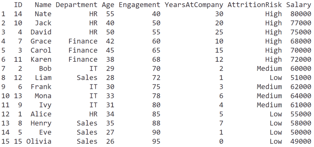
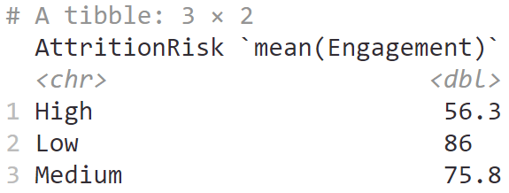
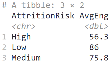
# Calculate mean engagement by attrition risk
summarise(group_by(hr_data, AttritionRisk),
          AvgEng = mean(Engagement))

ถ้าใช้ pipe operator แล้ว จะเขียนได้แบบนี้:

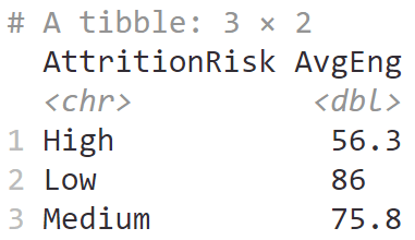
# Calculate mean engagement by attrition risk
hr_data |>
  
  # Group by AttritionRisk
  group_by(AttritionRisk) |>
  
  # Calculate mean
  summarise(AvgEng = mean(Engagement))

ซึ่ง code ทั้งสองชุดให้ผลลัพธ์ที่เหมือนกัน:

แต่จะเห็นได้ว่า code ที่ใช้ pipe operator มีความชัดเจนและอ่านง่ายกว่า เพราะไม่จำเป็นต้องเขียน code ที่ซ้อนกันเป็นชั้น ๆ

ทีนี้ ถ้าเราใช้ pipe operator เพื่อรวมทั้ง 5 functions เข้าด้วยกันแล้ว จะทำให้เราใช้ข้อมูลเพื่อตอบคำถามที่ซับซ้อนขึ้นได้

ตัวอย่าง:

ผู้บริหารอยากได้รายชื่อพนักงานในกลุ่มเสี่ยงลาออกสูง โดยเรียงตามอายุงานและเงินเดือน จากมากไปน้อย

เราสามารถใช้ pipe operator ร่วมกัน group_by() + summarise() + arrange() เพื่อตอบโจทย์ได้:

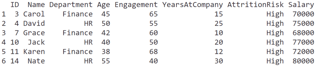
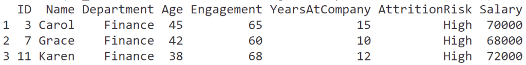
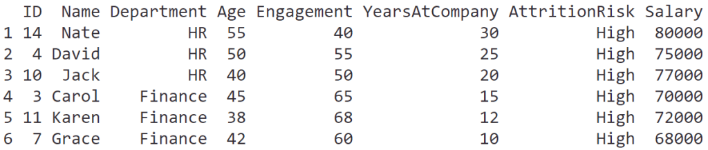
# Find employees with high attrition risk
# and sort by tenure and salary
hr_data |>
  
  # Filter for high attrition risk
  filter(AttritionRisk == "High") |>
  
  # Sort descending by tenure and salary
  arrange(desc(YearsAtCompany),
          desc(Salary))

ผลลัพธ์:

หรือ

ผู้บริหารต้องการรู้ว่า จำนวนพนักงานและค่าเฉลี่ยคะแนนการมีส่วนร่วมของแต่ละแผนก โดยเรียงแผนกจากค่าเฉลี่ยมากไปน้อย

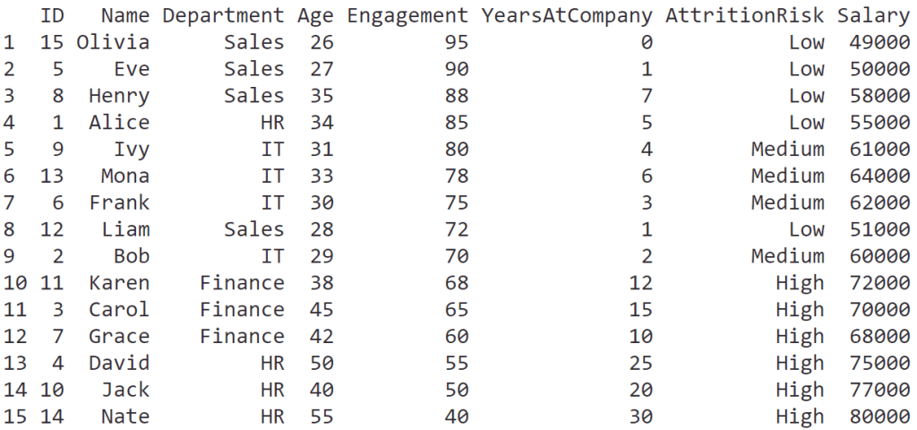
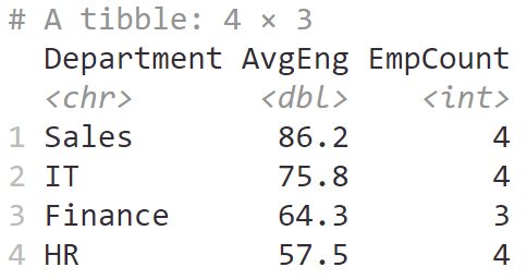
hr_data |> 
  
  # Group by department
  group_by(Department) |>
  
  # Calculate mean and count the number of employees
  summarise(AvgEng = mean(Engagement),
            EmpCount = n()) |>
  
  # Sort descending by average engagement
  arrange(desc(AvgEng))

ผลลัพธ์:

หรือ

ผู้บริหารต้องการรู้สัดส่วนพนักงานในกลุ่มความเสี่ยงสูงในแต่ละแผนก โดยเรียงจากมากไปน้อย และขอให้เรียงข้อมูลดังนี้: แผนก สัดส่วนเสี่ยงสูง จำนวนพนักงานทั้งหมด จำนวนพนักงานในกลุ่มเสี่ยงสูง

hr_data |>
  
  # Group by department
  group_by(Department) |>
  
  # Count high attrition risk and find attrition risk ratio
  summarise(HighRiskCount = sum(AttritionRisk == "High"),
            TotalEmp = n(),
            HighRiskRatio = (HighRiskCount / TotalEmp) * 100) |>
  
  # Select desired columns
  select(Department, HighRiskRatio, TotalEmp, HighRiskCount) |>
  
  # Sort descending by high rish ratio
  arrange(desc(HighRiskRatio))

ผลลัพธ์:

🔥 สรุป 5 Functions จาก dplyr

5 functions พื้นฐาน ของ dplyr เป็น functions ที่สามารถใช้ร่วมกันเพื่อทำงานกับข้อมูลต่าง ๆ เช่น ข้อมูลพนักงาน ได้อย่างมีประสิทธิภาพ

No.	Function	Explain
1	`select()`	เลือก column ที่ต้องการ
2	`filter()`	เลือก row ที่ต้องการ
3	`arrange()`	จัดลำดับข้อมูล
4	`sumamrise()`	สรุปข้อมูล
5	`mutate()`	แปลงข้อมูล

Note: ใช้ %>% หรือ |> เพื่อเชื่อม functions เข้าด้วยกัน

💪 Try It Yourself

สำหรับใครที่อยากลองเล่นใช้ R เล่นกับข้อมูล HR สามารถดาวน์โหลด code ตัวอย่างในบทความได้ที่ GitHub

📚 อ่านเพิ่มเติมเกี่ยวกับ dplyr

หนังสือ R for Data Science – สอนใช้ 5 functions ของ dplyr ด้วยชุดข้อมูล nycflights13 พร้อมแบบฝึกหัด: https://r4ds.hadley.nz/data-transform.html
Posit Cheatsheets – สรุปการใช้งาน 5 functions ของ dplyr: https://rstudio.github.io/cheatsheets/html/data-transformation.html
Official dplyr Documentation – คู่มืออย่างเป็นทางการในการใช้ 5 functions ของ dplyr: https://dplyr.tidyverse.org/

✅ R Book for Psychologists: หนังสือภาษา R สำหรับนักจิตวิทยา

📕 ขอฝากหนังสือเล่มแรกในชีวิตด้วยนะครับ 😆

Correlation
t-tests
ANOVA
Reliability
Factor analysis

แล้วทุกคนจะแปลกใจว่า ทำไมภาษา R ง่ายขนาดนี้ 🙂‍↕️

👉 สนใจดูรายละเอียดหนังสือได้ที่ meb:

ดูรายละเอียดหนังสือ R Book for Psychologists

2024-12-11

Tag: R

🧐 HCA คืออะไร?

💻 HCA ในภาษา R: hclust()

🔢 Example Dataset: USArrests

📏 Normalise the Data

🍿 HCA With hclust()

📈 Print & Dendrogram

😺 GitHub

📃 References

✅ R Book for Psychologists: หนังสือภาษา R สำหรับนักจิตวิทยา

Share this:

👉 Introduction to k-Means

🤔 k-Means คืออะไร?

🪜 Steps การทำงานของ k-Means

🏫 Learn More

💻 k-Means ในภาษา R: kmeans()

🔢 Dataset

🪨 rock

📏 Data Normalisation

🔎 Finding the Optimal k

⏹️ k-Means

🔥 Train the Model

🤓 Get the Results

😺 GitHub

📃 References

✅ R Book for Psychologists: หนังสือภาษา R สำหรับนักจิตวิทยา

Share this:

🌳 Tree-Based Algorithms คืออะไร?

💻 Tree-Based Models ในภาษา R

🚗 Dataset: mtcars

🔧 Prepare the Data

🪴 Train the Model

📏 Evaluate the Model

🍄 Random Forest

🐱 GitHub

📃 References

✅ R Book for Psychologists: หนังสือภาษา R สำหรับนักจิตวิทยา

Share this:

👼 Naïve Bayes คืออะไร?

🧑‍💻 วิธีสร้าง NB Classifer ด้วย naivebayes Package

1️⃣ Step 1. Install & Load the Package

2️⃣ Step 2. Load & Preview the Dataset

3️⃣ Step 3. Split the Dataset

4️⃣ Step 4. Create a NB Model

5️⃣ Step 5. Evaluate the Model

😺 GitHub

📃 References

✅ R Book for Psychologists: หนังสือภาษา R สำหรับนักจิตวิทยา

Share this:

💻 KNN in R With class Package

1️⃣ Step 1. Get class Package

2️⃣ Step 2. Get the Dataset

3️⃣ Step 3. Prepare Data

📉 Normalise Data

🪓 Split Data

🏷️ Separate Features From Label

4️⃣ Step 4. Train a KNN Model

5️⃣ Step 5. Evaluate the Model

🍩 Bonus: Fine-Tuning

😺 GitHub

📃 References

✅ R Book for Psychologists: หนังสือภาษา R สำหรับนักจิตวิทยา

Share this:

🏎️ dtplyr คืออะไร?

🧑‍💻 วิธีใช้ dytplyr

1️⃣ ขั้นที่ 1. Install & Load dtplyr

2️⃣ ขั้นที่ 2. Create a Lazy data.table

3️⃣ ขั้นที่ 3. Execute the Syntax

😺 GitHub

📃 References

✅ R Book for Psychologists: หนังสือภาษา R สำหรับนักจิตวิทยา

Share this:

🔤 gg for “Grammar of Graphics”

🏁 Getting Started With ggplot2

✍️ Basic Syntax

📊 Basic Plotting: Data, Aesthetics, & Geom

🎨 Aesthetics

⏹️ Geom

🔧 More Customisations

🖼️ Theme