Tag: R programming

สรุป 10 วิธีในการทำงานกับ data frame ในภาษา R: creating, indexing, subsetting, filtering, sorting, และอื่น ๆ — ตัวอย่างการทำงานกับ Jujutsu Kaisen data frame

Data frame เป็นหนึ่งใน data structure ที่พบบ่อยที่สุดในการทำงานกับข้อมูล

Data frame เก็บข้อมูลในรูปแบบตาราง โดย:

1 row = 1 รายการ (เช่น ข้อมูลของ John)
1 column = 1 ประเภทข้อมูล (เช่น อายุ)

ตัวอย่าง data frame:

ในบทความนี้ เราจะมาสรุป 10 วิธีในการทำงานกับ data frame กัน:

Creating: การสร้าง data frame
Previewing: การดูข้อมูล data frame
Indexing: การเลือก columns ที่ต้องการ
Subsetting: การเลือก rows และ columns ที่ต้องการ
Filtering: การกรองข้อมูล
Sorting: การจัดลำดับข้อมูล
Aggregating: การสรุปข้อมูล
Adding columns: การเพิ่ม columns ใหม่
Removing columns: การลบ columns
Binding: การเชื่อมข้อมูลใหม่เข้ากับ data frame

ถ้าพร้อมแล้ว ไปเริ่มกันเลย

1️⃣ Creating

เราสามารถสร้าง data frame ด้วย data.frame() ซึ่งต้องการ ชื่อ column และ vector ที่เก็บข้อมูลของ column นั้น ๆ:

# Create a data frame
jjk_df <- data.frame(
  ID = 1:10,
  Name = c("Yuji Itadori", "Megumi Fushiguro", "Nobara Kugisaki", "Satoru Gojo",
           "Maki Zenin", "Toge Inumaki", "Panda", "Kento Nanami", "Yuta Okkotsu", "Suguru Geto"),
  Age = c(15, 16, 16, 28, 17, 17, 18, 27, 17, 27),
  Grade = c("1st Year", "1st Year", "1st Year", "Special", "2nd Year",
            "2nd Year", "2nd Year", "Special", "Special", "Special"),
  CursedEnergy = c(80, 95, 70, 999, 60, 85, 75, 200, 300, 400),
  Technique = c("Divergent Fist", "Ten Shadows", "Straw Doll", "Limitless",
                "Heavenly Restriction", "Cursed Speech", "Gorilla Mode",
                "Ratio Technique", "Rika", "Cursed Spirit Manipulation"),
  Missions = c(25, 30, 20, 120, 35, 28, 40, 90, 55, 80)
)

# View the result
jjk_df

ผลลัพธ์:

   ID             Name Age    Grade CursedEnergy                  Technique Missions
1   1     Yuji Itadori  15 1st Year           80             Divergent Fist       25
2   2 Megumi Fushiguro  16 1st Year           95                Ten Shadows       30
3   3  Nobara Kugisaki  16 1st Year           70                 Straw Doll       20
4   4      Satoru Gojo  28  Special          999                  Limitless      120
5   5       Maki Zenin  17 2nd Year           60       Heavenly Restriction       35
6   6     Toge Inumaki  17 2nd Year           85              Cursed Speech       28
7   7            Panda  18 2nd Year           75               Gorilla Mode       40
8   8     Kento Nanami  27  Special          200            Ratio Technique       90
9   9     Yuta Okkotsu  17  Special          300                       Rika       55
10 10      Suguru Geto  27  Special          400 Cursed Spirit Manipulation       80

2️⃣ Previewing

เรามี 8 functions สำหรับดูข้อมูล data frame:

No.	Function	For
1	`View()`	ดูข้อมูลทั้งหมด
2	`head()`	ดูข้อมูล 6 rows แรก
3	`tail()`	ดูข้อมูล 6 rows สุดท้าย
4	`str()`	ดูโครงสร้างข้อมูล
5	`summary()`	ดูสถิติข้อมูล
6	`dim()`	ดูจำนวน rows และ columns
7	`nrow()`	ดูจำนวน rows
8	`ncol()`	ดูจำนวน columns

เราไปดูตัวอย่างทั้ง 8 functions กัน

👀 View()

View() ใช้ดูข้อมูลทั้งหมดใน data frame:

# View the whole data frame
View(jjk_df)

เราจะเห็นผลลัพธ์ในหน้าต่างใหม่:

Note: เนื่องจาก View() แสดงข้อมูลทั้งหมด จึงเหมาะกับการใช้งานกับ data frame ขนาดเล็ก

🙊 head()

head() ใช้ดูข้อมูล 6 rows แรกใน data frame:

# View the first 6 rows
head(jjk_df)

ผลลัพธ์:

  ID             Name Age    Grade CursedEnergy            Technique Missions
1  1     Yuji Itadori  15 1st Year           80       Divergent Fist       25
2  2 Megumi Fushiguro  16 1st Year           95          Ten Shadows       30
3  3  Nobara Kugisaki  16 1st Year           70           Straw Doll       20
4  4      Satoru Gojo  28  Special          999            Limitless      120
5  5       Maki Zenin  17 2nd Year           60 Heavenly Restriction       35
6  6     Toge Inumaki  17 2nd Year           85        Cursed Speech       28

🐒 tail()

tail() ใช้ดูข้อมูล 6 rows สุดท้ายใน data frame:

# View the last 6 rows
tail(jjk_df)

ผลลัพธ์:

   ID         Name Age    Grade CursedEnergy                  Technique Missions
5   5   Maki Zenin  17 2nd Year           60       Heavenly Restriction       35
6   6 Toge Inumaki  17 2nd Year           85              Cursed Speech       28
7   7        Panda  18 2nd Year           75               Gorilla Mode       40
8   8 Kento Nanami  27  Special          200            Ratio Technique       90
9   9 Yuta Okkotsu  17  Special          300                       Rika       55
10 10  Suguru Geto  27  Special          400 Cursed Spirit Manipulation       80

🏗️ str()

str() ใช้ดูโครงสร้างข้อมูลของ data frame:

# View the data frame structure
str(jjk_df)

ผลลัพธ์:

'data.frame':	10 obs. of  7 variables:
 $ ID          : int  1 2 3 4 5 6 7 8 9 10
 $ Name        : chr  "Yuji Itadori" "Megumi Fushiguro" "Nobara Kugisaki" "Satoru Gojo" ...
 $ Age         : num  15 16 16 28 17 17 18 27 17 27
 $ Grade       : chr  "1st Year" "1st Year" "1st Year" "Special" ...
 $ CursedEnergy: num  80 95 70 999 60 85 75 200 300 400
 $ Technique   : chr  "Divergent Fist" "Ten Shadows" "Straw Doll" "Limitless" ...
 $ Missions    : num  25 30 20 120 35 28 40 90 55 80

จากผลลัพธ์ เราจะเห็นข้อมูล 5 อย่าง ได้แก่:

จำนวน rows (obs.)
จำนวน columns (variables)
ชื่อ columns (เช่น ID)
ประเภทข้อมูลของแต่ละ column (เช่น int)
ตัวอย่างข้อมูลของแต่ละ column (เช่น 1 2 3 4 5 6 7 8 9 10)

🧮 summary()

summary() ใช้สรุปข้อมูลใน data frame เช่น:

ค่าเฉลี่ย (Mean)
จำนวนข้อมูล (Length)

# View the summary
summary(jjk_df)

ผลลัพธ์:

       ID            Name                Age           Grade            CursedEnergy     Technique            Missions     
 Min.   : 1.00   Length:10          Min.   :15.00   Length:10          Min.   : 60.00   Length:10          Min.   : 20.00  
 1st Qu.: 3.25   Class :character   1st Qu.:16.25   Class :character   1st Qu.: 76.25   Class :character   1st Qu.: 28.50  
 Median : 5.50   Mode  :character   Median :17.00   Mode  :character   Median : 90.00   Mode  :character   Median : 37.50  
 Mean   : 5.50                      Mean   :19.80                      Mean   :236.40                      Mean   : 52.30  
 3rd Qu.: 7.75                      3rd Qu.:24.75                      3rd Qu.:275.00                      3rd Qu.: 73.75  
 Max.   :10.00                      Max.   :28.00                      Max.   :999.00                      Max.   :120.00

💠 dim()

dim() ใช้แสดงจำนวน rows และ columns ใน data frame:

# View the dimensions
dim(jjk_df)

ผลลัพธ์:

[1] 10  7

🚣 nrow()

nrow() ใช้แสดงจำนวน rows ใน data frame:

# Get the number of rows
nrow(jjk_df)

ผลลัพธ์:

[1] 10

🏦 ncol()

ncol() ใช้แสดงจำนวน columns ใน data frame:

# Get the number of columns
ncol(jjk_df)

ผลลัพธ์:

[1] 7

3️⃣ Indexing

Indexing หมายถึง การเลือก columns ที่ต้องการ ซึ่งเราทำได้ 2 วิธี:

ใช้ $ (นิยมใช้)
ใช้ [[]]

💰 Using $

เราสามารถใช้ $ ได้แบบนี้:

df$col

ยกตัวอย่างเช่น เลือก column Name:

# Index with $
jjk_df$Name

ผลลัพธ์:

 [1] "Yuji Itadori"     "Megumi Fushiguro" "Nobara Kugisaki"  "Satoru Gojo"      "Maki Zenin"      
 [6] "Toge Inumaki"     "Panda"            "Kento Nanami"     "Yuta Okkotsu"     "Suguru Geto"

🔳 Using [[]]

เราสามารถใช้ [[]] ได้แบบนี้:

df[["col"]]

ยกตัวอย่างเช่น เลือก column Name:

# Index with [[]]
jjk_df[["Name"]]

ผลลัพธ์:

 [1] "Yuji Itadori"     "Megumi Fushiguro" "Nobara Kugisaki"  "Satoru Gojo"      "Maki Zenin"      
 [6] "Toge Inumaki"     "Panda"            "Kento Nanami"     "Yuta Okkotsu"     "Suguru Geto"

4️⃣ Subsetting

Subsetting คือ การเลือก rows และ columns จาก data frame ซึ่งเราทำได้ 2 วิธี:

ใช้ df[rows, cols] syntax
ใช้ subset()

🍽️ df[rows, cols]

เราสามารถใช้ df[rows, cols] ได้ 3 แบบ:

เลือก rows
เลือก columns
เลือก rows และ columns

แบบที่ 1. เลือก rows อย่างเดียว:

# Subset rows only
jjk_df[1:5, ]

ผลลัพธ์:

  ID             Name Age    Grade CursedEnergy            Technique Missions
1  1     Yuji Itadori  15 1st Year           80       Divergent Fist       25
2  2 Megumi Fushiguro  16 1st Year           95          Ten Shadows       30
3  3  Nobara Kugisaki  16 1st Year           70           Straw Doll       20
4  4      Satoru Gojo  28  Special          999            Limitless      120
5  5       Maki Zenin  17 2nd Year           60 Heavenly Restriction       35

แบบที่ 2. เลือก columns อย่างเดียว:

# Subset columns only
jjk_df[, "Name"]

ผลลัพธ์:

 [1] "Yuji Itadori"     "Megumi Fushiguro" "Nobara Kugisaki"  "Satoru Gojo"      "Maki Zenin"      
 [6] "Toge Inumaki"     "Panda"            "Kento Nanami"     "Yuta Okkotsu"     "Suguru Geto"

แบบที่ 3. เลือก rows และ columns:

# Subset rows and columns
jjk_df[1:5, c("Name", "Technique")]

ผลลัพธ์:

              Name            Technique
1     Yuji Itadori       Divergent Fist
2 Megumi Fushiguro          Ten Shadows
3  Nobara Kugisaki           Straw Doll
4      Satoru Gojo            Limitless
5       Maki Zenin Heavenly Restriction

🔪 subset()

เราสามารถ subset ข้อมูลได้ด้วย subset() ซึ่งต้องการ 2 arguemnts:

subset(x, select)

x = data frame
select = columns ที่ต้องการเลือก

# Subset using susbet() - select conlumns only
subset(jjk_df, select = c("Name", "Technique"))

ผลลัพธ์:

               Name                  Technique
1      Yuji Itadori             Divergent Fist
2  Megumi Fushiguro                Ten Shadows
3   Nobara Kugisaki                 Straw Doll
4       Satoru Gojo                  Limitless
5        Maki Zenin       Heavenly Restriction
6      Toge Inumaki              Cursed Speech
7             Panda               Gorilla Mode
8      Kento Nanami            Ratio Technique
9      Yuta Okkotsu                       Rika
10      Suguru Geto Cursed Spirit Manipulation

ในกรณีที่เราต้องการเลือก rows ด้วย เราจะต้องกำหนด rows ใน x:

# Subset using susbet() - select both rows and columns
subset(jjk_df[1:5, ], select = c("Name", "Technique"))

ผลลัพธ์:

              Name            Technique
1     Yuji Itadori       Divergent Fist
2 Megumi Fushiguro          Ten Shadows
3  Nobara Kugisaki           Straw Doll
4      Satoru Gojo            Limitless
5       Maki Zenin Heavenly Restriction

5️⃣ Filtering

เราสามารถกรองข้อมูลใน data frame ได้ 2 วิธี:

ใช้ df[rows, cols] syntax
ใช้ subset()

🍽️ df[rows, cols]

เราสามารถกรองข้อมูลด้วย df[rows, cols] โดยกำหนดเงื่อนไขการกรองใน rows

เช่น กรองข้อมูลตัวละครที่อยู่ปี 1:

# Filter using df[rows, cols] - 1 condition
jjk_df[jjk_df$Grade == "1st Year", ]

ผลลัพธ์:

  ID             Name Age    Grade CursedEnergy      Technique Missions
1  1     Yuji Itadori  15 1st Year           80 Divergent Fist       25
2  2 Megumi Fushiguro  16 1st Year           95    Ten Shadows       30
3  3  Nobara Kugisaki  16 1st Year           70     Straw Doll       20

ในกรณีที่เรามีมากกว่า 1 เงื่อนไข เราสามารถใช้ logical operators ช่วยได้:

Operator	Meaning
`&`	AND
`\|`	OR
`!`	NOT

ยกตัวอย่างเช่น กรองข้อมูลตัวละครที่อยู่ปี 1 และมีอายุ 15 ปี:

# Filter using df[rows, cols] - multiple conditions
jjk_df[jjk_df$Grade == "1st Year" & jjk_df$Age == 15, ]

ผลลัพธ์:

  ID         Name Age    Grade CursedEnergy      Technique Missions
1  1 Yuji Itadori  15 1st Year           80 Divergent Fist       25

🔪 subset()

เราสามารถใช้ subset() เพื่อกรองข้อมูลได้แบบนี้:

# Filter using sbuset() - 1 condition
subset(jjk_df, Grade == "1st Year")

ผลลัพธ์:

  ID             Name Age    Grade CursedEnergy      Technique Missions
1  1     Yuji Itadori  15 1st Year           80 Divergent Fist       25
2  2 Megumi Fushiguro  16 1st Year           95    Ten Shadows       30
3  3  Nobara Kugisaki  16 1st Year           70     Straw Doll       20

เราสามารถเพิ่มเงื่อนไขการกรองได้ด้วย logical operator เช่น:

# Filter using sbuset() - multiple conditions
subset(jjk_df, Grade == "1st Year" & Age == 15)

ผลลัพธ์:

  ID         Name Age    Grade CursedEnergy      Technique Missions
1  1 Yuji Itadori  15 1st Year           80 Divergent Fist       25

6️⃣ Sorting

สำหรับการเรียงข้อมูล เราจะใช้ order() ซึ่งเพื่อเรียงข้อมูลได้ 3 แบบ:

Ascending (A–Z)
Descending (Z–A)
Sort by multiple columns: จัดเรียงด้วยหลาย columns

⬇️ Ascending

ยกตัวอย่างเช่น เรียงลำดับตามจำนวนภารกิจ (Missions):

# Sort ascending (default)
jjk_df[order(jjk_df$Missions), ]

ผลลัพธ์:

   ID             Name Age    Grade CursedEnergy                  Technique Missions
3   3  Nobara Kugisaki  16 1st Year           70                 Straw Doll       20
1   1     Yuji Itadori  15 1st Year           80             Divergent Fist       25
6   6     Toge Inumaki  17 2nd Year           85              Cursed Speech       28
2   2 Megumi Fushiguro  16 1st Year           95                Ten Shadows       30
5   5       Maki Zenin  17 2nd Year           60       Heavenly Restriction       35
7   7            Panda  18 2nd Year           75               Gorilla Mode       40
9   9     Yuta Okkotsu  17  Special          300                       Rika       55
10 10      Suguru Geto  27  Special          400 Cursed Spirit Manipulation       80
8   8     Kento Nanami  27  Special          200            Ratio Technique       90
4   4      Satoru Gojo  28  Special          999                  Limitless      120

⬆️ Descending

เราสามารถเรียงข้อมูลแบบ descending ได้ 2 วิธี:

ใช้ decreasing
ใช้ -

วิธีที่ 1. ใช้ decreasing:

# Sort descending with decreasing
jjk_df[order(jjk_df$Missions, decreasing = TRUE), ]

ผลลัพธ์:

   ID             Name Age    Grade CursedEnergy                  Technique Missions
4   4      Satoru Gojo  28  Special          999                  Limitless      120
8   8     Kento Nanami  27  Special          200            Ratio Technique       90
10 10      Suguru Geto  27  Special          400 Cursed Spirit Manipulation       80
9   9     Yuta Okkotsu  17  Special          300                       Rika       55
7   7            Panda  18 2nd Year           75               Gorilla Mode       40
5   5       Maki Zenin  17 2nd Year           60       Heavenly Restriction       35
2   2 Megumi Fushiguro  16 1st Year           95                Ten Shadows       30
6   6     Toge Inumaki  17 2nd Year           85              Cursed Speech       28
1   1     Yuji Itadori  15 1st Year           80             Divergent Fist       25
3   3  Nobara Kugisaki  16 1st Year           70                 Straw Doll       20

วิธีที่ 2. ใช้ -:

# Sort descending with -
jjk_df[order(-jjk_df$Missions), ]

ผลลัพธ์:

   ID             Name Age    Grade CursedEnergy                  Technique Missions
4   4      Satoru Gojo  28  Special          999                  Limitless      120
8   8     Kento Nanami  27  Special          200            Ratio Technique       90
10 10      Suguru Geto  27  Special          400 Cursed Spirit Manipulation       80
9   9     Yuta Okkotsu  17  Special          300                       Rika       55
7   7            Panda  18 2nd Year           75               Gorilla Mode       40
5   5       Maki Zenin  17 2nd Year           60       Heavenly Restriction       35
2   2 Megumi Fushiguro  16 1st Year           95                Ten Shadows       30
6   6     Toge Inumaki  17 2nd Year           85              Cursed Speech       28
1   1     Yuji Itadori  15 1st Year           80             Divergent Fist       25
3   3  Nobara Kugisaki  16 1st Year           70                 Straw Doll       20

↔️ Sort by Multiple Columns

เราสามารถจัดเรียงข้อมูลได้มากกว่า 1 column ด้วยการเลือก columns ที่ต้องการจัดเรียงเพิ่ม

เช่น จัดเรียงด้วย:

Grade
จำนวนภารกิจ (Missions)

# Sort by mulitple columns
jjk_df[order(jjk_df$Grade, jjk_df$Missions), ]

ผลลัพธ์:

   ID             Name Age    Grade CursedEnergy                  Technique Missions
3   3  Nobara Kugisaki  16 1st Year           70                 Straw Doll       20
1   1     Yuji Itadori  15 1st Year           80             Divergent Fist       25
2   2 Megumi Fushiguro  16 1st Year           95                Ten Shadows       30
6   6     Toge Inumaki  17 2nd Year           85              Cursed Speech       28
5   5       Maki Zenin  17 2nd Year           60       Heavenly Restriction       35
7   7            Panda  18 2nd Year           75               Gorilla Mode       40
9   9     Yuta Okkotsu  17  Special          300                       Rika       55
10 10      Suguru Geto  27  Special          400 Cursed Spirit Manipulation       80
8   8     Kento Nanami  27  Special          200            Ratio Technique       90
4   4      Satoru Gojo  28  Special          999                  Limitless      120

7️⃣ Aggregating

เราสามารถสรุปข้อมูลโดยใช้ statistics functions เช่น:

Function	For
`mean()`	หาค่าเฉลี่ย
`median()`	หาค่ามัธยฐาน
`min()`	หาค่าต่ำสุด
`max()`	หาค่าสูงสุด
`sd()`	หาค่า standard deviation

ยกตัวอย่างเช่น หาค่าเฉลี่ย Cursed Energy (CursedEnergy):

# Find average Cursed Energy
mean(jjk_df$CursedEnergy)

ผลลัพธ์:

[1] 236.4

8️⃣ Adding Columns

เราสามารถเพิ่ม columns ใหม่ได้ด้วยแบบนี้:

df$new_col <- value

ยกตัวอย่างเช่น เพิ่ม column Ranking:

# Add a column
jjk_df$Ranking <- ifelse(jjk_df$CursedEnergy > 100, "High", "Low")

# View the result
jjk_df

ผลลัพธ์:

   ID             Name Age    Grade CursedEnergy                  Technique Missions Ranking
1   1     Yuji Itadori  15 1st Year           80             Divergent Fist       25     Low
2   2 Megumi Fushiguro  16 1st Year           95                Ten Shadows       30     Low
3   3  Nobara Kugisaki  16 1st Year           70                 Straw Doll       20     Low
4   4      Satoru Gojo  28  Special          999                  Limitless      120    High
5   5       Maki Zenin  17 2nd Year           60       Heavenly Restriction       35     Low
6   6     Toge Inumaki  17 2nd Year           85              Cursed Speech       28     Low
7   7            Panda  18 2nd Year           75               Gorilla Mode       40     Low
8   8     Kento Nanami  27  Special          200            Ratio Technique       90    High
9   9     Yuta Okkotsu  17  Special          300                       Rika       55    High
10 10      Suguru Geto  27  Special          400 Cursed Spirit Manipulation       80    High

9️⃣ Removing Columns

เราสามารถลบ columns ได้ด้วยวิธีเดียวกันกับการเพิ่ม columns:

df$col <- NULL

ยกตัวอย่างเช่น ลบ column Ranking:

# Remove a column
jjk_df$Ranking <- NULL

# View the result
jjk_df

ผลลัพธ์:

   ID             Name Age    Grade CursedEnergy                  Technique Missions
1   1     Yuji Itadori  15 1st Year           80             Divergent Fist       25
2   2 Megumi Fushiguro  16 1st Year           95                Ten Shadows       30
3   3  Nobara Kugisaki  16 1st Year           70                 Straw Doll       20
4   4      Satoru Gojo  28  Special          999                  Limitless      120
5   5       Maki Zenin  17 2nd Year           60       Heavenly Restriction       35
6   6     Toge Inumaki  17 2nd Year           85              Cursed Speech       28
7   7            Panda  18 2nd Year           75               Gorilla Mode       40
8   8     Kento Nanami  27  Special          200            Ratio Technique       90
9   9     Yuta Okkotsu  17  Special          300                       Rika       55
10 10      Suguru Geto  27  Special          400 Cursed Spirit Manipulation       80

🔟 Binding

เราสามารถเชื่อม data frame ได้ 2 แบบ:

rbind(): เชื่อม row
cbind(): เชื่อม column

🤝 rbind()

rbind() ใช้เชื่อม data frame กับ row ใหม่ และต้องการ 2 arguments:

rbind(df1, df2)

df1 = data frame ที่ 1
df2 = data frame ที่ 2

ยกตัวอย่างเช่น เพิ่มชื่อตัวละครใหม่ (Hajime Kashimo):

# Create a new data frame
new_sorcerer <- data.frame(
  ID = 11,
  Name = "Hajime Kashimo",
  Age = 25,
  Grade = "Special",
  CursedEnergy = 500,
  Technique = "Lightning",
  Missions = 60
)

# Bind the data frames by rows
jjk_df <- rbind(jjk_df, new_sorcerer)

# View the result
jjk_df

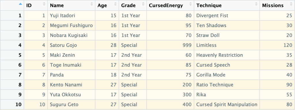
ผลลัพธ์:

   ID             Name Age    Grade CursedEnergy                  Technique Missions
1   1     Yuji Itadori  15 1st Year           80             Divergent Fist       25
2   2 Megumi Fushiguro  16 1st Year           95                Ten Shadows       30
3   3  Nobara Kugisaki  16 1st Year           70                 Straw Doll       20
4   4      Satoru Gojo  28  Special          999                  Limitless      120
5   5       Maki Zenin  17 2nd Year           60       Heavenly Restriction       35
6   6     Toge Inumaki  17 2nd Year           85              Cursed Speech       28
7   7            Panda  18 2nd Year           75               Gorilla Mode       40
8   8     Kento Nanami  27  Special          200            Ratio Technique       90
9   9     Yuta Okkotsu  17  Special          300                       Rika       55
10 10      Suguru Geto  27  Special          400 Cursed Spirit Manipulation       80
11 11   Hajime Kashimo  25  Special          500                  Lightning       60

🤲 cbind()

cbind() ใช้เชื่อม data frame กับ column ใหม่ และต้องการ 2 arguments ได้แก่:

cbind(df, vector)

df = data frame
vector = vector ที่เก็บข้อมูลของ column ใหม่

ยกตัวอย่างเช่น เพิ่ม column ที่บอกว่าตัวละครเป็นครูหรือไม่ (IsTeacher):

# Bind a column
jjk_df <- cbind(
  jjk_df,
  IsTeacher = c(FALSE, FALSE, FALSE, TRUE, FALSE,
                FALSE, FALSE, TRUE, FALSE, TRUE, FALSE)
)

# View the result
jjk_df

ผลลัพธ์:

   ID             Name Age    Grade CursedEnergy                  Technique Missions IsTeacher
1   1     Yuji Itadori  15 1st Year           80             Divergent Fist       25     FALSE
2   2 Megumi Fushiguro  16 1st Year           95                Ten Shadows       30     FALSE
3   3  Nobara Kugisaki  16 1st Year           70                 Straw Doll       20     FALSE
4   4      Satoru Gojo  28  Special          999                  Limitless      120      TRUE
5   5       Maki Zenin  17 2nd Year           60       Heavenly Restriction       35     FALSE
6   6     Toge Inumaki  17 2nd Year           85              Cursed Speech       28     FALSE
7   7            Panda  18 2nd Year           75               Gorilla Mode       40     FALSE
8   8     Kento Nanami  27  Special          200            Ratio Technique       90      TRUE
9   9     Yuta Okkotsu  17  Special          300                       Rika       55     FALSE
10 10      Suguru Geto  27  Special          400 Cursed Spirit Manipulation       80      TRUE
11 11   Hajime Kashimo  25  Special          500                  Lightning       60     FALSE

😺 GitHub

ดูตัวอย่าง code ทั้งหมดได้ที่ GitHub

📃 References

รูปประกอบจาก Jujutsu Kaisen Character Dataset
R Data Frames
DataFrame Operations in R

✅ R Book for Psychologists: หนังสือภาษา R สำหรับนักจิตวิทยา

📕 ขอฝากหนังสือเล่มแรกในชีวิตด้วยนะครับ 😆

🙋 ใครที่กำลังเรียนจิตวิทยาหรือทำงานสายจิตวิทยา และเบื่อที่ต้องใช้ software ราคาแพงอย่าง SPSS และ Excel เพื่อทำข้อมูล

💪 ผมขอแนะนำ R Book for Psychologists หนังสือสอนใช้ภาษา R เพื่อการวิเคราะห์ข้อมูลทางจิตวิทยา ที่เขียนมาเพื่อนักจิตวิทยาที่ไม่เคยมีประสบการณ์เขียน code มาก่อน

ในหนังสือ เราจะปูพื้นฐานภาษา R และพาไปดูวิธีวิเคราะห์สถิติที่ใช้บ่อยกัน เช่น:

Correlation
t-tests
ANOVA
Reliability
Factor analysis

🚀 เมื่ออ่านและทำตามตัวอย่างใน R Book for Psychologists ทุกคนจะไม่ต้องพึง SPSS และ Excel ในการทำงานอีกต่อไป และสามารถวิเคราะห์ข้อมูลด้วยตัวเองได้ด้วยความมั่นใจ

แล้วทุกคนจะแปลกใจว่า ทำไมภาษา R ง่ายขนาดนี้ 🙂‍↕️

👉 สนใจดูรายละเอียดหนังสือได้ที่ meb:

ดูรายละเอียดหนังสือ R Book for Psychologists

2025-12-11

Machine Learning in R: รวบรวม 13 บทความสอนสร้าง Machine Learning ในภาษา R
ภาษา R มี packages จำนวนมาก สำหรับสร้าง machine learning models

ในบทความนี้ ผมรวบรวม 13 บทความสอนทำ machine learning ซึ่งแบ่งได้เป็น 4 กลุ่ม ดังนี้:
1. Supervised learning models หรือการ train models แบบมีเฉลย
2. Tree-based models หรือการสร้าง model ที่ใช้ decision trees
3. Unsupervised learning models หรือการ train models แบบไม่มีเฉลย
4. All-in-one packages หรือ packages สำหรับทำ machine learning แบบครบครัน ตั้งแต่การเตรียมข้อมูลไปจนถึงการประเมินประสิทธิภาพ รวมทั้งใช้ model ได้ตามต้องการ
กลุ่มที่ 1. Supervised learning models (4 บทความ):
กลุ่มที่ 2. Tree-based models (3 บทความ):
กลุ่มที่ 3. Unsupervised learning models (3 บทความ):
กลุ่มที่ 4. All-in-one packages (2 บทความ):
1. caret (เป็น package ที่เก่ากว่า)
2. tidymodels (เป็น package ที่ใหม่กว่า)
Share this:
X
Facebook
Like Loading…
2025-12-06

7 วิธีทำงานกับ time series data ในภาษา R: Base R, lubridate, และ zoo packages — ตัวอย่างการวิเคราะห์ราคา Bitcoin

ในบทความนี้ เราจะมาเรียนรู้ 7 วิธีการทำงานกับ time series data หรือข้อมูลที่จัดเรียงด้วยเวลา ในภาษา R ผ่านการทำงานกับ Bitcoin Historical Data ซึ่งมีข้อมูล Bitcoin ในช่วงปี ค.ศ. 2010–2024 กัน:

Converting: การแปลงข้อมูลเป็น datetime และ time series
Missing values: การจัดการ missing values ใน time series data
Plotting: การสร้างกราฟ time series data
Subsetting: การเลือกข้อมูลจาก time series data
Aggregating: การสรุป time series data
Rolling window: การทำ rolling window
Expanding window: การทำ expanding window

ถ้าพร้อมแล้วไปเริ่มกันเลย

🏁 Getting Started

ในการเริ่มทำงานกับ time series ในภาษา R เราจะเริ่มต้นจาก 2 อย่าง ได้แก่:

Install and load packages
Load dataset

1️⃣ Install & Load Packages

ในภาษา R เรามี 3 packages ที่ใช้ทำงานกับ time series data บ่อย ๆ ได้แก่:

Base R packages ที่มาพร้อมกับภาษา R
lubridate: ใช้แปลงข้อมูลและจัด format ของ date-time data
zoo: ใช้ทำงานกับ time series data

ในการเริ่มต้นใช้งาน เราจะติดตั้ง packages เหล่านี้กัน:

# Install packages
install.packages("lubridate"
install.packages("zoo")
install.packages("ggplot2") # for data visualisation

จากนั้น เรียกใช้งาน packages:

# Load packages
library(lubridate)
library(zoo)
library(ggplot2) # for data visualisation

Note: เราเพิ่ม ggplot2 เข้ามาด้วย เพื่อช่วยในการสร้างกราฟในภายหลัง

2️⃣ Load Dataset

หลังติดตั้งและเรียกใช้งาน packages เราจะโหลด Bitcoin Historical Data (ดาวน์โหลดไฟล์ได้ที่ Kaggle) เข้ามาใน environment:

# Load the dataset
btc <- read.csv("btc_hist_2010-2024.csv")

จากนั้น เราสามารถสำรวจข้อมูลได้ด้วย head() และ str():

## View the first 6 rows
head(btc)

## View the structure
str(btc)

ผลลัพธ์ของ head():

          Date    Price     Open     High      Low   Vol. Change..
1 Feb 09, 2024 47,545.4 45,293.3 47,710.2 45,254.2 86.85K    4.97%
2 Feb 08, 2024 45,293.3 44,346.2 45,579.2 44,336.4 66.38K    2.15%
3 Feb 07, 2024 44,339.8 43,088.4 44,367.9 42,783.5 48.57K    2.91%
4 Feb 06, 2024 43,087.7 42,697.6 43,375.5 42,566.8 33.32K    0.91%
5 Feb 05, 2024 42,697.2 42,581.4 43,532.2 42,272.5 39.26K    0.27%
6 Feb 04, 2024 42,581.4 43,006.2 43,113.2 42,379.4 20.33K   -0.99%

ผลลัพธ์ของ str():

'data.frame':	4955 obs. of  7 variables:
 $ Date    : chr  "Feb 09, 2024" "Feb 08, 2024" "Feb 07, 2024" "Feb 06, 2024" ...
 $ Price   : chr  "47,545.4" "45,293.3" "44,339.8" "43,087.7" ...
 $ Open    : chr  "45,293.3" "44,346.2" "43,088.4" "42,697.6" ...
 $ High    : chr  "47,710.2" "45,579.2" "44,367.9" "43,375.5" ...
 $ Low     : chr  "45,254.2" "44,336.4" "42,783.5" "42,566.8" ...
 $ Vol.    : chr  "86.85K" "66.38K" "48.57K" "33.32K" ...
 $ Change..: chr  "4.97%" "2.15%" "2.91%" "0.91%" ...

จากผลลัพธ์ เราจะเห็นว่า Bitcoin Historical Data มี 7 columns ด้วยกัน ได้แก่:

No.	Column	Description
1	`Date`	วันที่
2	`Close`	ราคาปิด (USD)
3	`Open`	ราคาเปิด (USD)
4	`High`	ราคาสูงสุด (USD)
5	`Low`	ราคาต่ำสุด (USD)
6	`Vol.`	ปริมาณการซื้อขาย
7	`Change..`	การเปลี่ยนแปลงราคาจากวันก่อน (คิดเป็น %)

นอกจากนี้ เราจะเห็นได้ว่า ทุก column เป็น character ซึ่งเราจะต้องแปลงให้เป็นประเภทข้อมูลที่ถูกต้องก่อน ซึ่งเราสามารถทำได้ดังนี้:

สร้าง copy ของ btc
เปลี่ยนชื่อ column (เพื่อให้ง่ายต่อการทำงาน)
เปลี่ยน format ข้อมูลของ price และ volume
แปลงประเภทข้อมูลจาก character เป็น numeric

# Clean the dataset

## Make a copy of the dataset
btc_cleaned <- btc

## Rename columns

### Create new column names
new_col_names <- c("date",
                   "close", "open",
                   "high", "low",
                   "volume", "change")

### Rename
colnames(btc_cleaned) <- new_col_names

### Check the results
str(btc_cleaned)

## Convert data types

### Specify the columns to clean
cols_to_clean <- c("close", "open",
                   "high", "low")

### Remove comma
for (col in cols_to_clean) {
  btc_cleaned[[col]] <- gsub(",",
                             "",
                             btc_cleaned[[col]])
}

### Remove "K"
btc_cleaned$volume <- gsub("K",
                           "",
                           btc_cleaned$volume)

### Remove "%"
btc_cleaned$change <- gsub("%",
                           "",
                           btc_cleaned$change)

### Specify columns to convert to numeric
cols_to_num <- colnames(btc_cleaned[, -1])

### Convert data type to numeric
for (col in cols_to_num) {
  btc_cleaned[[col]] <- as.numeric(btc_cleaned[[col]])
}

### Check the results
str(btc_cleaned)

ผลลัพธ์:

'data.frame':	4955 obs. of  7 variables:
 $ date  : chr  "Feb 09, 2024" "Feb 08, 2024" "Feb 07, 2024" "Feb 06, 2024" ...
 $ close : num  47545 45293 44340 43088 42697 ...
 $ open  : num  45293 44346 43088 42698 42581 ...
 $ high  : num  47710 45579 44368 43376 43532 ...
 $ low   : num  45254 44336 42784 42567 42273 ...
 $ volume: num  86.8 66.4 48.6 33.3 39.3 ...
 $ change: num  4.97 2.15 2.91 0.91 0.27 -0.99 -0.44 0.26 1.18 -0.85 ...

ตอนนี้ ทุก column (ยกเว้น date) ถูกเปลี่ยนให้เป็น numeric เรียบร้อยแล้ว และชุดข้อมูลก็พร้อมจะถูกนำไปใช้งานต่อแล้ว

🔄️ Converting

เรามาดูวิธีแรกในการทำงานกับ time series data กัน นั่นคือ:

การแปลงข้อมูลให้เป็น datetime
การแปลงข้อมูลให้เป็น time series

1️⃣ การแปลงข้อมูลให้เป็น Datetime

ในการทำงานกับ time series data เราจะต้องแปลงข้อมูลประเภทอื่น ๆ เช่น character และ numeric ให้เป็น datetime ก่อน เช่น date (เช่น “Feb 09, 2024”) ใน Bitcoin dataset

เราสามารถแปลงข้อมูลจาก character เป็น Date ได้ 2 วิธี ดังนี้:

วิธีที่ 1. ใช้ as.Date() ซึ่งเป็น base R function และต้องการ input 2 อย่าง ได้แก่:

x: ข้อมูลที่ต้องการแปลงเป็น Date
format: format ของวันเวลาของข้อมูลต้นทาง (เช่น วัน-เดือน-ปี, ปี-เดือน-วัน, เดือน-วัน-ปี)

# Convert `date` to Date
btc_cleaned$date <- as.Date(btc_cleaned$date,
                            format = "%b %d, %Y")

Note: ศึกษาการกำหนด format ได้ที่ strptime: Date-time Conversion Functions to and from Character และ Date Formats in R

วิธีที่ 2. ใช้ as_date() จาก lubridate ซึ่งเป็นที่นิยมมากกว่า as.Date() เพราะ as_date() แปลงข้อมูลให้อัตโนมัติ โดยเราไม่ต้องกำหนด format ให้:

# Convert `date` to Date
btc_cleaned$date <- as_date(btc_cleaned$date)

จากตัวอย่าง จะเห็นได้ว่า as_date() ใช้งานง่ายกว่า as.Date()

ทั้งนี้ ทั้งสองวิธีให้ผลลัพธ์เหมือนกัน คือ แปลง character เป็น Date ซึ่งเราสามารถเช็กผลลัพธ์ได้ด้วย str():

# Check the results
str(btc_cleaned)

ผลลัพธ์:

'data.frame':	4955 obs. of  7 variables:
 $ date  : Date, format: "2024-02-09" "2024-02-08" "2024-02-07" ...
 $ close : num  47545 45293 44340 43088 42697 ...
 $ open  : num  45293 44346 43088 42698 42581 ...
 $ high  : num  47710 45579 44368 43376 43532 ...
 $ low   : num  45254 44336 42784 42567 42273 ...
 $ volume: num  86.8 66.4 48.6 33.3 39.3 ...
 $ change: num  4.97 2.15 2.91 0.91 0.27 -0.99 -0.44 0.26 1.18 -0.85 ...

จะเห็นได้ว่า ตอนนี้ price เปลี่ยนเป็นจาก character เป็น Date เรียบร้อยแล้ว

2️⃣ การแปลงข้อมูลให้เป็น Time Series

นอกจากการแปลงข้อมูลบางส่วนให้เป็น datetime แล้ว เรายังต้องการแปลง dataset จาก data frame ให้เป็น time series เพื่อมี index ของข้อมูล เป็น datetime

ในภาษา R เรามี time series 2 ประเภทหลัก ได้แก่:

ts ของ base R ซึ่งเหมาะกับข้อมูลที่มีความถี่คงที่ (เช่น ข้อมูลมีระยะห่างกัน 1 วัน)
zoo จาก zoo package ซึ่งเหมาะกับข้อมูลที่มีความถี่ไม่คงที่ (เช่น บางข้อมูลห่างกัน 1 วัน และบางข้อมูลห่างกัน 1 เดือน)

ในตัวอย่าง Bitcoin เราจะแปลง dataset ให้เป็น zoo กัน:

# Convert data frame to zoo object

## Convert
btc_zoo <- zoo(btc_cleaned[, -1],
               order.by = btc_cleaned$date)

## Check the results
head(btc_zoo)

ผลลัพธ์:

           close open high low volume change
2010-07-18   0.1  0.0  0.1 0.1   0.08      0
2010-07-19   0.1  0.1  0.1 0.1   0.57      0
2010-07-20   0.1  0.1  0.1 0.1   0.26      0
2010-07-21   0.1  0.1  0.1 0.1   0.58      0
2010-07-22   0.1  0.1  0.1 0.1   2.16      0
2010-07-23   0.1  0.1  0.1 0.1   2.40      0

จะเห็นได้ว่า datetime ถูกเปลี่ยนให้เป็น index ของข้อมูลแล้ว

🤷‍♂️ Missing Values

ในบางครั้ง เราอาจมี time series data ที่มีข้อมูลขาดหายไป ซึ่งเราอาจต้องการแทนที่ด้วยค่าบางอย่าง

ในตัวอย่าง Bitcoin dataset เรามี missing values อยู่ใน volume ซึ่งเราสามารถเช็กได้ด้วย colSums() และ is.na() แบบนี้:

# Count the missing values in each column
colSums(is.na(btc_zoo))

ผลลัพธ์:

 close   open   high    low volume change 
     0      0      0      0    271      0

zoo package มี 3 functions ที่ช่วยให้เราแทนค่า missing values ได้ ดังนี้:

No.	Function	Description
1	`na.fill()`	แทนค่าด้วยค่าที่เรากำหนด
2	`na.locf()`	แทนค่าตามค่าของข้อมูลที่มาก่อนหน้า
3	`na.approx()`	แทนค่าด้วยตามข้อมูลที่มาก่อนและหลัง missing values

สำหรับ Bitcoin dataset เราจะใช้ na.approx() เนื่องจากข้อมูล Bitcoin มีความผันผวนและการแทนค่าแบบยืดหยุ่นจะดีกว่าการแทนค่าแบบกำหนดตายตัว:

# Impute with na.approx()
btc_zoo <- na.approx(btc_zoo)

# Check the results
colSums(is.na(btc_zoo))

ผลลัพธ์:

 close   open   high    low volume change 
     0      0      0      0      0      0

ตอนนี้ missing values ถูกแทนค่าเรียบร้อย

📈 Plotting

การสร้างกราฟสามารถช่วยให้เราเข้าใจ time series data ได้ง่ายขึ้น

เราสามารถทำได้ง่าย ๆ ด้วย autoplot.*() เช่น autoplot.ts() และ autplot.zoo()

ใน Bitcoin dataset เราสามารถสร้างกราฟราคาปิดของ Bitcoin ในช่วง 2010**–**2024 ได้ด้วย autoplot.zoo() แบบนี้:

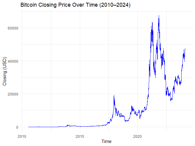
# Plot the time series
autoplot.zoo(btc_zoo[, "close"]) +
  
  ## Adjust line colour
  geom_line(color = "blue") +
  
  ## Add title and labels
  labs(title = "Bitcoin Closing Price Over Time (2010–2024)",
       x = "Time",
       y = "Closing Price (USD)") +
  
  ## Use minimal theme
  theme_minimal()

ผลลัพธ์:

Note: ในตัวอย่าง เราใช้ ggplot2 ช่วยตกแต่งกราฟให้เข้าใจง่ายขึ้น, สำหรับคนที่สนใจ สามารถศึกษาการใช้ ggplot2 ได้ที่ วิธีใช้ ggplot2 เพื่อสร้างกราฟอย่างมืออาชีพระดับโลก แบบ BBC และ Financial Times ในภาษา R — ตัวอย่างการสำรวจข้อมูลเพนกวินจาก palmerpenguins

✂️ Subsetting

ในการทำงานกับ time series data เราอาจต้องการตัดแบ่งข้อมูลบางส่วนมาเพื่อสำรวจการเปลี่ยนแปลงของข้อมูลในช่วงเวลาที่ต้องการ

ยกตัวอย่างเช่น เราอยากจะสำรวจการเปลี่ยนแปลงราคาปิดของ Bitcoin ในช่วง Crypto Winter (Nov 2021 – Dec 2022)

ในภาษา R เราสามารถตัดแบ่ง time series ได้ 3 วิธี ได้แก่:

window()
Boolean masking
Specific date

1️⃣ window()

window() เป็น base R function ซึ่งช่วยเราเลือกช่วงเวลาได้ด้วย input 3 อย่าง:

x: time series data
start: วันเริ่มต้น (inclusive)
end: วันสิ้นสุด (inclusive)

เราสามารถใช้ window() สร้างกราฟได้แบบนี้:

# Subset
btc_winter_1 <- window(x = btc_zoo,
                       start = as.Date("2021-11-01"),
                       end = as.Date("2022-12-31"))

# Plot the results
autoplot.zoo(btc_winter_1[, "close"]) +
  
  ## Adjust line colour
  geom_line(color = "blue") +
  
  ## Add title and labels
  labs(title = "Bitcoin Closing Price During the Crypto Winter (2021–2022)",
       x = "Time",
       y = "Closing (USD)") +
  
  ## Use minimal theme
  theme_minimal()

ผลลัพธ์:

2️⃣ Boolean Masking

นอกจาก window() แล้ว เราสามารถเลือกช่วงเวลาด้วยการสร้าง Boolean mask ขึ้นมา แบบนี้:

# Create a Boolean masking
crypto_winter_index <- 
  index(btc_zoo) >= "2021-11-01" &
  index(btc_zoo) <= "2022-12-31"

# Subset
btc_winter_2 <- btc_zoo[crypto_winter_index, ]

# Plot the results
autoplot.zoo(btc_winter_2[, "close"]) +  
  
  ## Adjust line colour
  geom_line(color = "blue") +
  
  ## Add title and labels
  labs(title = "Bitcoin Closing Price During the Crypto Winter (2021–2022)",
       x = "Time",
       y = "Closing (USD)") +
  
  ## Use minimal theme
  theme_minimal()

ผลลัพธ์:

จะเห็นว่า กราฟของ Boolean masking เหมือนกับการใช้ window()

3️⃣ Specific Date

ในกรณีที่เราต้องการเลือกวันแทนช่วงเวลา (เช่น ดูข้อมูล Bitcoin เมื่อเกิด halving ครั้งแรก) เราสามารถเขียนภาษา R ได้แบบนี้:

# Subset
btc_first_halving <- btc_zoo["2012-11-28"]

# Print the result
btc_first_halving

ผลลัพธ์:

           close open high  low volume change
2012-11-28  12.4 12.2 12.4 12.1  30.69   1.23

🧮 Aggregating

ในภาษา R เราสามารถสรุปข้อมูล time series data (เช่น หาค่าเฉลี่ย) ได้ด้วย apply.*() จาก zoo package:

Function	Description
`apply.daily()`	สรุปข้อมูลรายวัน
`apply.weekly()`	สรุปข้อมูลรายสัปดาห์
`apply.quarterly()`	สรุปข้อมูลรายไตรมาส
`apply.yearly()`	สรุปข้อมูลรายปี

โดย apply.*() ต้องการ input 2 อย่าง คือ:

x: time series data
FUN: การสรุปข้อมูล (เช่น mean, median, max, min)

ยกตัวอย่างเช่น หาค่าเฉลี่ยราคาปิดของ Bitcoin ในแต่ละปี:

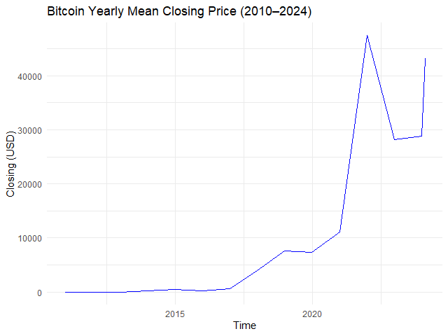
# Example 1. View yearly mean closing price
btc_yr_mean <- apply.yearly(btc_zoo[, "close"],
                            FUN = mean)

# Plot the results
autoplot.zoo(btc_yr_mean) +  
  
  ## Adjust line colour
  geom_line(color = "blue") +
  
  ## Add title and labels
  labs(title = "Bitcoin Yearly Mean Closing Price (2010–2024)",
       x = "Time",
       y = "Closing (USD)") +
  
  ## Use minimal theme
  theme_minimal()

ผลลัพธ์:

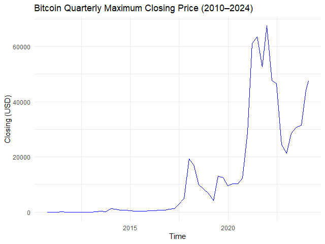
หรือหาราคาปิดสูงสุดในแต่ละไตรมาส:

# Example 2. View quarterly max closing price
btc_qtr_max <- apply.quarterly(btc_zoo[, "close"],
                               FUN = max)

# Plot the results
autoplot.zoo(btc_qtr_max) +  
  
  ## Adjust line colour
  geom_line(color = "blue") +
  
  ## Add title and labels
  labs(title = "Bitcoin Quarterly Maximum Closing Price (2010–2024)",
       x = "Time",
       y = "Closing (USD)") +
  
  ## Use minimal theme
  theme_minimal()

ผลลัพธ์:

ทั้งนี้ ถ้าเราต้องการกำหนดความถี่ของเวลาเอง เราสามารถใช้ endpoints() คู่กับ period.apply() ได้

โดย endpoints() ต้องการ input 3 อย่าง:

x: time series data
on: ระดับช่วงเวลา (เช่น ปี, เดือน, สัปดาห์)
k: จำนวน

และ period.apply() ต้องการ input 3 อย่าง คือ:

x: time series data
INDEX: variable ที่เก็บ endpoints() เอาไว้
FUN: function ที่ใช้สรุปข้อมูล (เช่น mean())

ยกตัวอย่างเช่น เราต้องการหาค่าเฉลี่ยราคาปิด Bitcoin ทุก ๆ 3 เดือน เราจะเขียนภาษา R ได้แบบนี้:

# Create 3-month interval
three_month_eps <- endpoints(x = btc_zoo,
                             on = "months",
                             k = 3)

# Apply the interval
btc_three_month_data <- period.apply(x = btc_zoo[, "close"],
                                     INDEX = three_month_eps,
                                     FUN = mean)

# Plot the results
autoplot.zoo(btc_three_month_data) +  
  
  ## Adjust line colour
  geom_line(color = "blue") +
  
  ## Add title and labels
  labs(title = "Bitcoin 3-Month Average Closing Price (2010–2024)",
       x = "Date",
       y = "Closing Price (USD)") +
  
  ## Use minimal theme
  theme_minimal()

ผลลัพธ์:

🪟 Rolling Window

Rolling window (moving window หรือ sliding window) คือ การสรุปข้อมูลตามช่วงเวลาที่กำหนด โดยช่วงเวลาในการคำนวณจะเคลื่อนตัวไปเรื่อย ๆ

เช่น เราต้องการหาค่าเฉลี่ยของราคาปิด Bitcoin ในช่วง 7 วันล่าสุด การใช้ rolling window จะทำให้เราได้ข้อมูลดังนี้:

Date	Average
2024-01-07	ค่าเฉลี่ยระหว่างวันที่ 1 ถึง 7
2024-01-08	ค่าเฉลี่ยระหว่างวันที่ 2 ถึง 8
2024-01-09	ค่าเฉลี่ยระหว่างวันที่ 3 ถึง 9

ในภาษา R เราสามารถสร้าง rolling window ได้ 2 วิธี:

ใช้ roll*()
ใช้ rollapply()

**1️⃣ roll*()**

เราสามารถสร้าง rolling window ได้ด้วย roll*() จาก zoo package เช่น:

Function	Description
`rollmean()`	หาค่าเฉลี่ย
`rollmedian()`	หาค่ากลาง
`rollmax()`	หาค่าสูงสุด
`rollsum()`	หาผลรวม

roll*() ต้องการ input 3 อย่าง ได้แก่:

x: time series data
k: ช่วงเวลา (window)
align: กำหนดว่า ค่าสรุปที่ได้จะอยู่ด้วยซ้าย ขวา หรือกลางช่วงเวลา
fill: จะแทนค่า missing values หรือไม่

ยกตัวอย่างเช่น เราต้องการหาค่าเฉลี่ยราคาปิด Bitcoin ในช่วง 30 วัน เราจะใช้ rollmean() แบบนี้:

# Create the window for mean price
btc_30_days_roll_mean <- rollmean(x = btc_zoo,
                                  k = 30,
                                  align = "right",
                                  fill = NA)

# Plot the results
autoplot.zoo(btc_30_days_roll_mean[, "close"]) +  
  
  ## Adjust line colour
  geom_line(color = "blue") +
  
  ## Add title and labels
  labs(title = "Bitcoin 30-Day Rolling Mean Price (2010–2024)",
       x = "Time",
       y = "Closing (USD)") +
  
  ## Use minimal theme
  theme_minimal()

ผลลัพธ์:

2️⃣ rollapply()

ในกรณีที่เราต้องการกำหนดการสรุปข้อมูลใน rolling window (เช่น หาค่าต่ำสุด ซึ่งไม่มีใน zoo package) เราสามารถทำได้ด้วย rollapply() ซึ่งต้องการ input 4 อย่างดังนี้:

data: time series data
width: ช่วงเวลา (window)
FUN: การสรุปข้อมูล (เช่น min)
align: กำหนดว่า ค่าสรุปที่ได้จะอยู่ด้วยซ้าย ขวา หรือกลางช่วงเวลา
fill: จะแทนค่า missing values หรือไม่

ยกตัวอย่างเช่น หาราคาปิดต่ำสุดของทุก ๆ 30 วัน:

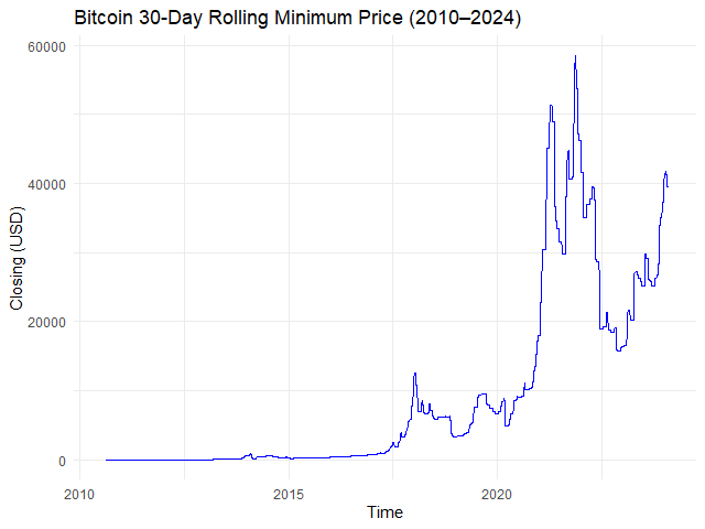
# Creating a rolling window with min() function
btc_30_days_roll_min <- rollapply(data = btc_zoo,
                                  width = 30,
                                  FUN = min,
                                  align = "right",
                                  fill = NA)

# Plot the results
autoplot.zoo(btc_30_days_roll_min[, "close"]) +  
  
  ## Adjust line colour
  geom_line(color = "blue") +
  
  ## Add title and labels
  labs(title = "Bitcoin 30-Day Rolling Minimum Price (2010–2024)",
       x = "Time",
       y = "Closing (USD)") +
  
  ## Use minimal theme
  theme_minimal()

ผลลัพธ์:

➡️ Expanding Window

Expanding window เป็นการสรุปข้อมูลแบบสะสม เช่น:

Date	Average
2024-01-01	หาค่าเฉลี่ยของวันที่ 1
2024-01-02	หาค่าเฉลี่ยของวันที่ 1 + 2
2024-01-03	หาค่าเฉลี่ยของวันที่ 1 + 2 + 3
2024-01-04	หาค่าเฉลี่ยของวันที่ 1 + 2 + 3 + 4
2024-01-05	หาค่าเฉลี่ยของวันที่ 1 + 2 + 3 + 4 + 5

ในภาษา R เราสามารถสร้าง expanding window ได้ด้วย rollapply() โดยเราต้องกำหนดให้:

width เป็นชุดตัวเลข (เช่น 1, 2, 3, …)
align = "right" เสมอ

ยกตัวอย่างเช่น สร้าง expanding window แบบค่าเฉลี่ยราคาปิดของเดือนมกราคม 2024:

# Subset for Jan 2024 data
btc_jan_2024 <- window(x = btc_zoo,
                       start = as.Date("2024-01-01"),
                       end = as.Date("2024-01-31"))

# Create a sequence of widths
btc_jan_2024_width <- seq_along(btc_jan_2024)

# Create an expanding window for mean price
btc_exp_mean <- rollapply(data = btc_2024,
                          width = btc_jan_2024_width,
                          FUN = mean,
                          align = "right",
                          fill = NA)

# Plot the results
autoplot.zoo(btc_exp_mean[, "close"]) +  
  
  ## Adjust line colour
  geom_line(color = "blue") +
  
  ## Add title and labels
  labs(title = "Bitcoin Expanding Mean Price (Jan 2024)",
       x = "Time",
       y = "Closing (USD)") +
  
  ## Use minimal theme
  theme_minimal()

ผลลัพธ์:

😎 Summary

ในบทความนี้ เราได้ทำความรู้จักกับ 7 วิธีการทำงานกับ time series ในภาษา R โดยใช้ base R, lubridate, และ zoo package กัน:

วิธีการทำงาน 1. Converting:

Function	For
`as.Date()`	แปลง character เป็น Date
`as_date()`	แปลง character เป็น Date
`zoo()`	แปลง data frame เป็น `zoo`

วิธีการทำงาน #2. Missing values:

Function	For
`na.fill()`	แทนค่า missing values ด้วยค่าที่กำหนด
`na.locf()`	แทนค่า missing values ตามค่าของข้อมูลที่มาก่อนหน้า
`na.approx()`	แทนค่า missing values ด้วยการวิเคราะห์ข้อมูลที่มาก่อนและหลัง missing values

วิธีการทำงาน #3. Plotting:

Function	For
`autoplot.zoo()`	สร้างกราฟจาก `zoo`

วิธีการทำงาน #4. Subsetting:

Function	For
`window()`	ดึงข้อมูลช่วงเวลาที่ต้องการ
`btc_zoo[boolean_mask, ]`	ดึงข้อมูลช่วงเวลาที่ต้องการ
`btx_zoo[x, y]`	ดึงข้อมูลวันที่ต้องการ

วิธีการทำงาน #5. Aggregating:

Function	For
`apply.daily()`	สรุปข้อมูลรายวัน
`apply.weekly()`	สรุปข้อมูลรายสัปดาห์
`apply.quarterly()`	สรุปข้อมูลรายไตรมาส
`apply.yearly()`	สรุปข้อมูลรายปี
`endpoints()` และ `period.apply()`	สรุปข้อมูลตามช่วงเวลาที่กำหนดเอง

วิธีการทำงาน #6. Rolling window:

Function	For
`rollmean()`	rolling window แบบหาค่าเฉลี่ย
`rollmedian()`	rolling window แบบหาค่ากลาง
`rollmax()`	rolling window แบบหาค่าสูงสุด
`rollsum()`	rolling window แบบหาผลรวม
`rollapply()`	rolling window แบบกำหนดการสรุปข้อมูลเอง

วิธีการทำงาน #7. Expanding window:

Function	For
`seq_along()` และ `rollapply()`	สร้าง expanding window

😺 View Code in GitHub

ดู code และ dataset ในบทความนี้ได้ที่ GitHub

📃 References

✅ R Book for Psychologists: หนังสือภาษา R สำหรับนักจิตวิทยา

📕 ขอฝากหนังสือเล่มแรกในชีวิตด้วยนะครับ 😆

Correlation
t-tests
ANOVA
Reliability
Factor analysis

แล้วทุกคนจะแปลกใจว่า ทำไมภาษา R ง่ายขนาดนี้ 🙂‍↕️

👉 สนใจดูรายละเอียดหนังสือได้ที่ meb:

ดูรายละเอียดหนังสือ R Book for Psychologists

2025-07-17

สอนปลูกต้นไม้ในภาษา R (ภาค 3): 5 ขั้นตอนการสร้าง Boosted Trees ด้วย xgboost package ในภาษา R — ตัวอย่างการทำนายระดับการกินน้ำมันของรถใน mpg dataset
ในบทความนี้ เราจะไปทำความรู้จักกับ eXtreme Gradient Boosting (XGBoost) และวิธีสร้าง XGBoost model ในภาษา R ด้วย xgboost package กัน

ถ้าพร้อมแล้ว ไปเริ่มกันเลย
อ่านเกี่ยวกับการปลูกต้นไม้ในภาษา R ภาคก่อน ๆ ได้ที่:
- ภาค 1: ปลูกด้วย rpart และ randomForest packages
- ภาค 2: ปลูกด้วย ranger package
🚀 XGBoost คืออะไร?

XGBoost เป็น machine learning model ที่จัดอยู่ในกลุ่ม tree-based models หรือ models ที่ทำนายข้อมูลด้วย decision tree อย่าง single decision tree และ random forest

ใน XGBoost, decision trees จะถูกสร้างขึ้นมาเป็นรอบ ๆ โดยในแต่ละรอบ decision trees ใหม่จะเรียนรู้จากความผิดพลาดของรอบก่อน ซึ่งจะทำให้ decision trees ใหม่มีความสามารถที่ดีขึ้นเรื่อย ๆ

เมื่อสิ้นสุดการสร้าง XGBoost ใช้ผลรวมของ decision trees ทุกต้นในการทำนายข้อมูล ดังนี้:
- Regression problem: หาค่าเฉลี่ยแบบถ่วงน้ำหนักจากทุกต้น
- Classification problem: ทำนายผลลัพธ์ด้วยค่าเฉลี่ยความน่าจะเป็นจากทุกต้น
💻 XGBoost ในภาษา R

ในภาษา R เราสามารถสร้าง XGBoost ได้ด้วย xgboost package ใน 5 ขั้นตอน ได้แก่:
1. Install and load the package
2. Load and prepare the data
3. Split the data
4. Train the model
5. Evaluate the model
1️⃣ Install & Load the Package

ในขั้นแรก ให้เราติดตั้งและเรียกใช้งาน xgboost package

ติดตั้ง:
```
# Install
install.packages("xgboost")
```
เรียกใช้งาน:
```
# Load
library(xgboost)
```
2️⃣ Load & Prepare the Data

ในขั้นตอนที่สอง ให้เราโหลดและเตรียมข้อมูลที่จะใช้สร้าง XGBoost model โดยในบทความนี้ เราจะใช้ mpg dataset จาก ggplot2 package กัน

mpg ประกอบด้วยข้อมูลรถและระดับการใช้น้ำมัน และจุดประสงค์ของเรา คือ ทำนายระดับการกินน้ำมันเมื่อรถวิ่งบน highway (hwy)

เราสามารถโหลด mpg ได้ผ่าน ggplot2:
```
# Install ggplot2
install.packages("ggplot2")

# Load ggplot2
library(ggplot2)

# Load the dataset
data(mpg)
```
เมื่อโหลด dataset แล้ว เราสามารถสำรวจข้อมูลได้ด้วย head():
```
# Preview
head(mpg)
```
ผลลัพธ์:
```
# A tibble: 6 × 11
  manufacturer model displ  year   cyl trans      drv     cty   hwy fl    class  
  <chr>        <chr> <dbl> <int> <int> <chr>      <chr> <int> <int> <chr> <chr>  
1 audi         a4      1.8  1999     4 auto(l5)   f        18    29 p     compact
2 audi         a4      1.8  1999     4 manual(m5) f        21    29 p     compact
3 audi         a4      2    2008     4 manual(m6) f        20    31 p     compact
4 audi         a4      2    2008     4 auto(av)   f        21    30 p     compact
5 audi         a4      2.8  1999     6 auto(l5)   f        16    26 p     compact
6 audi         a4      2.8  1999     6 manual(m5) f        18    26 p     compact
```
และดูโครงสร้างข้อมูลด้วย str():
```
# View the tructure
str(mpg)
```
ผลลัพธ์:
```
tibble [234 × 11] (S3: tbl_df/tbl/data.frame)
 $ manufacturer: chr [1:234] "audi" "audi" "audi" "audi" ...
 $ model       : chr [1:234] "a4" "a4" "a4" "a4" ...
 $ displ       : num [1:234] 1.8 1.8 2 2 2.8 2.8 3.1 1.8 1.8 2 ...
 $ year        : int [1:234] 1999 1999 2008 2008 1999 1999 2008 1999 1999 2008 ...
 $ cyl         : int [1:234] 4 4 4 4 6 6 6 4 4 4 ...
 $ trans       : chr [1:234] "auto(l5)" "manual(m5)" "manual(m6)" "auto(av)" ...
 $ drv         : chr [1:234] "f" "f" "f" "f" ...
 $ cty         : int [1:234] 18 21 20 21 16 18 18 18 16 20 ...
 $ hwy         : int [1:234] 29 29 31 30 26 26 27 26 25 28 ...
 $ fl          : chr [1:234] "p" "p" "p" "p" ...
 $ class       : chr [1:234] "compact" "compact" "compact" "compact" ...
```
จากผลลัพธ์ เราจะเห็นได้ว่า mpg มี columns ที่เราต้องปรับจาก character เป็น factor อยู่ เช่น manufacturer, model ซึ่งเราสามารถปรับได้ดังนี้:
```
# Convert character columns to factor

## Get character columns
chr_cols <- c("manufacturer",
              "model",
              "trans",
              "drv",
              "fl",
              "class")

## For-loop through the character columns
for (col in chr_cols) {
  mpg[[col]] <- as.factor(mpg[[col]])
}

## Check the results
str(mpg)
```
ผลลัพธ์:
```
tibble [234 × 11] (S3: tbl_df/tbl/data.frame)
 $ manufacturer: Factor w/ 15 levels "audi","chevrolet",..: 1 1 1 1 1 1 1 1 1 1 ...
 $ model       : Factor w/ 38 levels "4runner 4wd",..: 2 2 2 2 2 2 2 3 3 3 ...
 $ displ       : num [1:234] 1.8 1.8 2 2 2.8 2.8 3.1 1.8 1.8 2 ...
 $ year        : int [1:234] 1999 1999 2008 2008 1999 1999 2008 1999 1999 2008 ...
 $ cyl         : int [1:234] 4 4 4 4 6 6 6 4 4 4 ...
 $ trans       : Factor w/ 10 levels "auto(av)","auto(l3)",..: 4 9 10 1 4 9 1 9 4 10 ...
 $ drv         : Factor w/ 3 levels "4","f","r": 2 2 2 2 2 2 2 1 1 1 ...
 $ cty         : int [1:234] 18 21 20 21 16 18 18 18 16 20 ...
 $ hwy         : int [1:234] 29 29 31 30 26 26 27 26 25 28 ...
 $ fl          : Factor w/ 5 levels "c","d","e","p",..: 4 4 4 4 4 4 4 4 4 4 ...
 $ class       : Factor w/ 7 levels "2seater","compact",..: 2 2 2 2 2 2 2 2 2 2 ...
```
ตอนนี้ columns ที่เราต้องการถูกเปลี่ยนเป็น factor เรียบร้อยแล้ว

3️⃣ Split the Data

ในขั้นที่สาม เราจะทำ 3 อย่างด้วยกัน คือ:
1. แยกตัวแปรต้น (x) และตัวแปรตาม (y) ออกจากกัน
2. แบ่งข้อมูลออกเป็น training และ test sets
3. แปลงข้อมูลให้เป็น DMatrix
ข้อที่ 1. เราสามารถแยกตัวแปรต้นและตัวแปรตามออกจากกันได้ดังนี้:
```
# Separate the features from the outcome

## Get the features
x <- mpg[, !names(mpg) %in% "hwy"]

## One-hot encode the features
x <- model.matrix(~ . - 1,
                  data = x)

## Get the outcome
y <- mpg$hwy
```
สังเกตว่า ตอนที่เราแยกตัวแปรต้น เราแปลงตัวแปรเหล่านี้เป็น 0, 1 ด้วย one-hot encoding ด้วย เนื่องจาก xgboost ต้องการตัวแปรต้นที่เป็น numeric

.

ข้อที่ 2. จากนั้น เราจะแบ่ง dataset เป็น training (80%) และ test sets (20%) ดังนี้:
```
# Split the data

## Set seed for reproducibility
set.seed(360)

## Get training index
train_index <- sample(1:nrow(x),
                      nrow(x) * 0.8)

## Create x, y train
x_train <- x[train_index, ]
y_train <- y[train_index]

## Create x, y test
x_test <- x[-train_index, ]
y_test <- y[-train_index]

## Check the results
cat("TRAIN SET", "\\n")
cat("1. Data in x_train:", nrow(x_train), "\\n")
cat("2. Data in y_train:", length(y_train), "\\n")
cat("---", "\\n", "TEST SET", "\\n")
cat("1. Data in x_test:", nrow(x_test), "\\n")
cat("2. Data in y_test:", length(y_test), "\\n")
```
ผลลัพธ์:
```
TRAIN SET
1. Data in x_train: 187
2. Data in y_train: 187
---
TEST SET
1. Data in x_test: 47
2. Data in y_test: 47
```
.

ข้อที่ 3. สุดท้าย เราจะแปลง x, y เป็น DMatrix ซึ่งเป็น object ที่ xgboost ใช้ในการสร้าง XGboost model ดังนี้:
```
# Convert to DMatrix

## Training set
train_set <- xgb.DMatrix(data = x_train,
                         label = y_train)

## Test set
test_set <- xgb.DMatrix(data = x_test,
                        label = y_test)

## Check the results
train_set
test_set
```
ผลลัพธ์:
```
TRAIN SET
xgb.DMatrix  dim: 187 x 77  info: label  colnames: yes
---
TEST SET
xgb.DMatrix  dim: 47 x 77  info: label  colnames: yes
```
4️⃣ Train the Model

ในขั้นที่สี่ เราจะสร้าง XGBoost model ด้วย xgb.train() ซึ่งต้องการ 5 arguments ดังนี้:
```
xgb.train(params, data, nrounds, watchlist, verbose)
```
1. params = hyperparametre ที่ต้องการใช้สร้าง model ที่ดีที่สุด
2. data = training set ที่ใช้สร้าง model
3. nrounds = จำนวนครั้งในการในสร้าง decision trees
4. watchlist = ชุดข้อมูลที่ต้องการใช้ประเมินความสามารถของ model
5. verbose = พิมพ์ข้อมูลในระหว่างการสร้าง model (1) หรือไม่ (0)
(Note: ศึกษา argument อื่น ๆ ของ xgb.train() ได้ที่ XGBoost Parameters)

สำหรับบทความนี้ เราจะใช้ xgb.train() ดังนี้:
```
# Train the model

## Set hyperparametres
hp <- list(objective = "reg:squarederror",
           eta = 0.1,
           max_depth = 4,
           eval_metric = c("rmse",
                           "mae"))

## Train
xgb_model <- xgb.train(params = hp,
                       data = train_set,
                       nrounds = 50,
                       watchlist = list(train = train_set,
                                        test = test_set),
                       verbose = 1)
```
ผลลัพธ์:
```
[1]	train-rmse:21.083975	test-rmse:22.739357 
[2]	train-rmse:19.045063	test-rmse:20.598582 
[3]	train-rmse:17.204130	test-rmse:18.713079 
[4]	train-rmse:15.549113	test-rmse:16.974701 
[5]	train-rmse:14.053049	test-rmse:15.453560 
[6]	train-rmse:12.707307	test-rmse:14.097377 
[7]	train-rmse:11.495216	test-rmse:12.877722 
[8]	train-rmse:10.402476	test-rmse:11.767320 
[9]	train-rmse:9.413522	test-rmse:10.740546 
[10]	train-rmse:8.525230	test-rmse:9.863130 
[11]	train-rmse:7.722776	test-rmse:9.068840 
[12]	train-rmse:7.000648	test-rmse:8.357181 
[13]	train-rmse:6.346603	test-rmse:7.687483 
[14]	train-rmse:5.758685	test-rmse:7.091249 
[15]	train-rmse:5.229548	test-rmse:6.557082 
[16]	train-rmse:4.753713	test-rmse:6.079389 
[17]	train-rmse:4.325653	test-rmse:5.651858 
[18]	train-rmse:3.940325	test-rmse:5.275154 
[19]	train-rmse:3.594545	test-rmse:4.938849 
[20]	train-rmse:3.283961	test-rmse:4.627743 
[21]	train-rmse:3.003089	test-rmse:4.352060 
[22]	train-rmse:2.747553	test-rmse:4.110172 
[23]	train-rmse:2.519617	test-rmse:3.889650 
[24]	train-rmse:2.314957	test-rmse:3.691806 
[25]	train-rmse:2.133630	test-rmse:3.499208 
[26]	train-rmse:1.969083	test-rmse:3.330280 
[27]	train-rmse:1.823011	test-rmse:3.181541 
[28]	train-rmse:1.693565	test-rmse:3.045308 
[29]	train-rmse:1.575817	test-rmse:2.919070 
[30]	train-rmse:1.469256	test-rmse:2.812063 
[31]	train-rmse:1.375599	test-rmse:2.700515 
[32]	train-rmse:1.292928	test-rmse:2.615973 
[33]	train-rmse:1.218867	test-rmse:2.541929 
[34]	train-rmse:1.151134	test-rmse:2.462113 
[35]	train-rmse:1.092395	test-rmse:2.404873 
[36]	train-rmse:1.039158	test-rmse:2.336600 
[37]	train-rmse:0.993882	test-rmse:2.291398 
[38]	train-rmse:0.952062	test-rmse:2.236936 
[39]	train-rmse:0.915935	test-rmse:2.198657 
[40]	train-rmse:0.879957	test-rmse:2.152984 
[41]	train-rmse:0.850423	test-rmse:2.102272 
[42]	train-rmse:0.822475	test-rmse:2.054172 
[43]	train-rmse:0.799025	test-rmse:2.011621 
[44]	train-rmse:0.775398	test-rmse:1.971787 
[45]	train-rmse:0.755066	test-rmse:1.933539 
[46]	train-rmse:0.736655	test-rmse:1.900084 
[47]	train-rmse:0.719087	test-rmse:1.870832 
[48]	train-rmse:0.705279	test-rmse:1.853400 
[49]	train-rmse:0.691914	test-rmse:1.834918 
[50]	train-rmse:0.680016	test-rmse:1.825738 
```
จะเห็นได้ว่า model ในแต่ละรอบมี RMSE หรือตัวบ่งชี้ความคลาดเคลื่อน ที่ลดลงเรื่อย ๆ เนื่องจาก model ใหม่เรียนรู้จากความผิดพลาดของ model ก่อนหน้า

หลังจากสร้าง model เสร็จแล้ว เราสามารถดูรายละเอียดของ model ได้แบบนี้:
```
# Print the model
xgb_model
```
ผลลัพธ์:
```
##### xgb.Booster
raw: 62.4 Kb 
call:
  xgb.train(params = hp, data = train_set, nrounds = 50, watchlist = list(train = train_set, 
    test = test_set), verbose = 1)
params (as set within xgb.train):
  objective = "reg:squarederror", eta = "0.1", max_depth = "4", eval_metric = "rmse", validate_parameters = "mae", objective = "TRUE"
xgb.attributes:
  niter
callbacks:
  cb.print.evaluation(period = print_every_n)
  cb.evaluation.log()
# of features: 77 
niter: 50
nfeatures : 77 
evaluation_log:
  iter train_rmse test_rmse
 <num>      <num>     <num>
     1 21.0839746 22.739357
     2 19.0450628 20.598582
   ---        ---       ---
    49  0.6919137  1.834918
    50  0.6800159  1.825738
```
5️⃣ Evaluate the Model

ในขั้นสุดท้าย เราจะประเมินความสามารถของ model ใน 3 ขั้นตอนกัน คือ:
1. ใช้ model ทำนายตัวแปรตาม
2. คำนวณ MAE, RMSE, และ R squared
3. Print MAE, RMSE, และ R squared
.

ข้อที่ 1. ใช้ model ทำนายตัวแปรตาม ด้วย predict():
```
# Make predictions
y_pred <- predict(xgb_model,
                  newdata = x_test)

# Compare predictions to actual outcomes
results <- data.frame(actual = y_test,
                      predicted = y_pred,
                      error = y_test - y_pred)

# Preview the results
head(results, 10)
```
ผลลัพธ์:
```
   actual predicted      error
1      31  27.81219  3.1878090
2      25  25.89449 -0.8944893
3      30  30.13318 -0.1331844
4      29  26.77814  2.2218552
5      24  24.34723 -0.3472347
6      23  23.58175 -0.5817528
7      19  17.81131  1.1886921
8      12  12.32908 -0.3290768
9      12  12.31534 -0.3153391
10     16  16.25793 -0.2579288
```
.

ข้อที่ 2. คำนวณ MAE, RMSE, และ R squared ซึ่งเป็นตัวชี้วัดความสามารถของ regression models:
```
# Calculate MAE
mae <- mean(abs(results$error))

# Calculate RMSE
rmse <- sqrt(mean((results$error)^2))

# Calculate R squared
ss_res <- sum((results$error)^2)
ss_tot <- sum((results$actual - mean(results$actual))^2)
r_squared <- 1 - (ss_res / ss_tot)
```
.

ข้อที่ 3. แสดงผลลัพธ์:
```
# Print the results
cat("MAE:", round(mae, 2), "\\n")
cat("RMSE:", round(rmse, 2), "\\n")
cat("R squared:", round(r_squared, 2), "\\n")
```
ผลลัพธ์:
```
MAE: 1.23
RMSE: 1.83
R squared: 0.93 
```
จะเห็นได้ว่า model ของเราสามารถอธิบายตัวแปรตามได้ถึง 93% (R squared) และมีความคลาดเคลื่อนโดยเฉลี่ย 1.23 miles per gallon (MAE)

💪 Summary

ในบทความนี้ เราได้ไปทำความรู้จักการสร้าง boosted tree ด้วย xgboost package ในภาษา R ซึ่งมีการทำงาน 5 ขั้นตอนกัน:
1. Install and load the package
2. Load and prepare the data
3. Split the data
4. Train the model
5. Evaluate the model
😺 GitHub

ดู code ทั้งหมดในบทความนี้ได้ที่ GitHub

📃 References
✅ R Book for Psychologists: หนังสือภาษา R สำหรับนักจิตวิทยา

📕 ขอฝากหนังสือเล่มแรกในชีวิตด้วยนะครับ 😆

🙋 ใครที่กำลังเรียนจิตวิทยาหรือทำงานสายจิตวิทยา และเบื่อที่ต้องใช้ software ราคาแพงอย่าง SPSS และ Excel เพื่อทำข้อมูล

💪 ผมขอแนะนำ R Book for Psychologists หนังสือสอนใช้ภาษา R เพื่อการวิเคราะห์ข้อมูลทางจิตวิทยา ที่เขียนมาเพื่อนักจิตวิทยาที่ไม่เคยมีประสบการณ์เขียน code มาก่อน

ในหนังสือ เราจะปูพื้นฐานภาษา R และพาไปดูวิธีวิเคราะห์สถิติที่ใช้บ่อยกัน เช่น:
- Correlation
- t-tests
- ANOVA
- Reliability
- Factor analysis
🚀 เมื่ออ่านและทำตามตัวอย่างใน R Book for Psychologists ทุกคนจะไม่ต้องพึง SPSS และ Excel ในการทำงานอีกต่อไป และสามารถวิเคราะห์ข้อมูลด้วยตัวเองได้ด้วยความมั่นใจ

แล้วทุกคนจะแปลกใจว่า ทำไมภาษา R ง่ายขนาดนี้ 🙂‍↕️

👉 สนใจดูรายละเอียดหนังสือได้ที่ meb:

ดูรายละเอียดหนังสือ R Book for Psychologists
Share this:
X
Facebook
Like Loading…
2025-07-03

Generalised Linear Model: วิธีใช้ glm() ในภาษา R เพื่อทำนายข้อมูลที่ไม่ปกติ — Linear, Logistic, และ Poisson Regression

ในบทความนี้ เราจะไปทำความรู้จักกับ generalised linear model (GLM) และวิธีทำ GLM ในภาษา R กัน

ถ้าพร้อมแล้ว ไปเริ่มกันเลย

🤔 GLM คืออะไร?

GLM เป็นเทคนิคทางสถิติที่ใช้ทำนายข้อมูลที่มีการกระจายตัวไม่ปกติ (non-normal distribution) เช่น ข้อมูลที่มีผลลัพธ์เพียง 0 และ 1

GLM ทำนายข้อมูลเหล่านี้โดยการต่อยอดจากสมการเส้นตรง (linear model) และมี 3 องค์ประกอบ ได้แก่:

Family: การกระจายตัวของตัวแปรตาม (y)
Linear predictors: สมการเส้นตัวตรงของตัวแปรต้น (x) หรือตัวแปรทำนาย (predictor)
Link function: function ที่เชื่อมตัวแปรต้นกับตัวแปรตามเข้าด้วยกัน

💻 GLM ในภาษา R

ในภาษา R เราสามารถใช้งาน GLM ได้ผ่าน glm() function ซึ่งต้องการข้อมูล 3 อย่าง:

glm(formula, data, family)

formula = ความสัมพันธ์ระหว่างตัวแปรต้นและตัวแปรตาม ในรูปแบบ y ~ x
data = ชุดข้อมูลที่ใช้ในการวิเคราะห์
family = การกระจายตัวของตัวแปรตาม

จะสังเกตว่า glm() ไม่มี parametre สำหรับ link function ทั้งนี้เป็นเพราะ glm() เรียกใช้ link function ให้อัตโนมัติตาม family ที่เรากำหนด

ทั้งนี้ ประเภทข้อมูล, family, และ link function ที่เราสามารถเรียกใช้ glm() ได้มีดังนี้:

Data	family	Link Function
Normal	`gaussian`	`link = "identity”`
Binomial	`binomial`	`link = "logit”`
Poisson	`poisson`	`link = "log”`
Quasi-poisson	`quasipoisson`	`link = "log”`
Gamma	`Gamma`	`link = "inverse”`

เราไปดูตัวอย่างการใช้งาน glm() เพื่อทำนายและแปลผลกัน

☕ ตัวอย่างข้อมูล: coffee_shop

เราจะไปดูตัวอย่างการใช้ glm() เพื่อทำนายข้อมูล 3 ประเภทกัน:

Linear regression
Logistic regression
Poisson regression

โดยเราจะใช้ตัวอย่างเป็นข้อมูลจำลองชื่อ coffee_shop ซึ่งประกอบด้วยข้อมูลการขายจากร้านกาแฟแห่งหนึ่ง และมีรายละเอียดดังนี้:

No.	Column	Description
1	`day`	วันที่
2	`temp`	อุณหภูมิโดยเฉลี่ยของวัน
3	`promo`	เป็นวันที่มีโปรโมชัน (มี, ไม่มี)
4	`weekend`	เป็นวันหยุดสุดสัปดาห์ (วันหยุด, วันธรรมดา)
5	`sales`	ยอดขาย
6	`customers`	จำนวนลูกค้าในแต่ละวัน
7	`sold_out`	ขายหมด (หมด, ไม่หมด)

ก่อนวิเคราะห์ข้อมูล เราจะสร้าง coffee_shop ตามนี้:

# Generate mock coffee shop dataset (15 days)

## Set seed for reproducibility
set.seed(123)

## Generate
coffee_shop <- data.frame(
  
  ## Generate 15 days
  day = 1:15,
  
  ## Generate daily temperature
  temp = round(rnorm(15,
                     mean = 25,
                     sd = 5),
               1),
  
  ## Generate promotion day
  promo = sample(c(0, 1),
                 15,
                 replace = TRUE),
  
  ## Generate weekend
  weekend = c(0, 0, 0, 0, 1, 1, 0, 0, 0, 1, 1, 0, 0, 0, 1),
  
  ## Generate the number of sales
  sales = round(rnorm(15,
                      mean = 300,
                      sd = 50)),
  
  ## Generate the number of daily customers
  customers = rpois(15,
                    lambda = 80),
  
  ## Generate sold-out
  sold_out = sample(c(0, 1),
                    15,
                    replace = TRUE)
)

## Convert binary variables to factors
coffee_shop$promo <- factor(coffee_shop$promo,
                            levels = c(0, 1),
                            labels = c("NoPromo", "Promo"))

coffee_shop$weekend <- factor(coffee_shop$weekend,
                              levels = c(0, 1),
                              labels = c("Weekday", "Weekend"))

coffee_shop$sold_out <- factor(coffee_shop$sold_out,
                               levels = c(0, 1),
                               labels = c("No", "Yes"))

## View the dataset
print(coffee_shop)

ผลลัพธ์:

   day temp   promo weekend sales customers sold_out
1    1 22.2 NoPromo Weekday   246        73      Yes
2    2 23.8   Promo Weekday   296        76      Yes
3    3 32.8 NoPromo Weekday   354        83       No
4    4 25.4   Promo Weekday   293        87       No
5    5 25.6   Promo Weekend   242        78      Yes
6    6 33.6 NoPromo Weekend   259        91      Yes
7    7 27.3 NoPromo Weekday   334        71      Yes
8    8 18.7 NoPromo Weekday   284        76       No
9    9 21.6 NoPromo Weekday   234        72      Yes
10  10 22.8   Promo Weekend   270        79       No
11  11 31.1 NoPromo Weekend   294        82      Yes
12  12 26.8   Promo Weekday   344        79       No
13  13 27.0   Promo Weekday   292        79       No
14  14 25.6 NoPromo Weekday   316        92       No
15  15 22.2 NoPromo Weekend   139        77      Yes

เราไปดูวิธีทำนายข้อมูลกัน

1️⃣ Linear Regression

Linear regression เป็นการทำนายข้อมูล numeric เช่น ยอดขาย (sales) ซึ่งเราสามารถใช้ glm() ทำนายได้ดังนี้:

# Create a regression model with glm()
linear_reg <- glm(sales ~ temp + promo + weekend,
                  data = coffee_shop,
                  family = gaussian)

เราสามารถดู model ได้ด้วย summary():

# Get model summary
summary(linear_reg)

ผลลัพธ์:

Call:
glm(formula = sales ~ temp + promo + weekend, family = gaussian, 
    data = coffee_shop)

Coefficients:
               Estimate Std. Error t value Pr(>|t|)   
(Intercept)      96.599     59.669   1.619  0.13375   
temp              7.703      2.283   3.373  0.00621 **
promoPromo       23.014     18.537   1.241  0.24025   
weekendWeekend  -73.444     19.654  -3.737  0.00328 **
---
Signif. codes:  0 ‘***’ 0.001 ‘**’ 0.01 ‘*’ 0.05 ‘.’ 0.1 ‘ ’ 1

(Dispersion parameter for gaussian family taken to be 1222.243)

    Null deviance: 39702  on 14  degrees of freedom
Residual deviance: 13445  on 11  degrees of freedom
AIC: 154.54

Number of Fisher Scoring iterations: 2

จากผลลัพธ์ เราจะเห็นความสำคัญของตัวแปรต้นและ coefficient ซึ่งระบุการเปลี่ยนแปลงของตัวแปรตามการเปลี่ยนของตัวแปรต้น:

ตัวแปรที่สามารถทำนาย sales ได้อย่างมีนัยสำคัญ คือ temp และ weekend (สังเกตจาก **)
promo ไม่สามารถทำนาย sales ได้อย่างมีนัยสำคัญ
Coefficient ของ temp คือ 7.70 ซึ่งหมายถึง อุณหภูมิเปลี่ยน 1 หน่วย ยอดขายจะเพิ่มขึ้น 7.70 หน่วย
Coefficient ของ weekend คือ -73.44 ซึ่งหมายถึง วันหยุดสุดสัปดาห์ ยอดขายจะลดลง 73.44 หน่วย

2️⃣ Logistic Regression

Logistic regression เป็นการทำนายข้อมูลที่เป็นมีผลลัพธ์เพียง 2 ค่า เช่น:

ใช่, ไม่ใช่
ผ่าน, ไม่ผ่าน
ตรง, ไม่ตรง

ใน coffee_shop เรามี sold_out ซึ่งเราสามารถทำนายด้วย logistic regression ด้วย glm() ได้แบบนี้:

# Create a logistic regression model
log_reg <- glm(sold_out ~ temp + promo + weekend,
               data = coffee_shop,
               family = binomial)

จากนั้น ดู model ด้วย summary():

# Get model summary
summary(log_reg)

ผลลัพธ์:

Call:
glm(formula = sold_out ~ temp + promo + weekend, family = binomial, 
    data = coffee_shop)

Coefficients:
               Estimate Std. Error z value Pr(>|z|)
(Intercept)     1.30934    3.92442   0.334    0.739
temp           -0.04448    0.15189  -0.293    0.770
promoPromo     -1.73681    1.31881  -1.317    0.188
weekendWeekend  2.15038    1.45643   1.476    0.140

(Dispersion parameter for binomial family taken to be 1)

    Null deviance: 20.728  on 14  degrees of freedom
Residual deviance: 16.426  on 11  degrees of freedom
AIC: 24.426

Number of Fisher Scoring iterations: 4

จะเห็นได้ว่า หน้าตาผลลัพธ์คล้ายกับ linear regression แต่สิ่งที่แตกต่างกัน คือ coefficient อยู่ในรูป log-odd ซึ่งเราสามารถถอดรูปได้ด้วย exp() เพื่อแปลผล:

# Transform coefficient
exp(coef(log_reg))

ผลลัพธ์:

   (Intercept)           temp     promoPromo weekendWeekend 
     3.7037124      0.9564938      0.1760812      8.5881237

เราสามารถแปลผลได้ดังนี้:

Predictor	Coefficient	Interpretation
`temp`	0.96	เมื่ออุณหภูมิสูงขึ้น 1 หน่วย ร้านมีโอกาสขายหมดเพิ่มขึ้น 0.96
`promo`	0.18	เมื่อมีโปรโมชัน ร้านมีโอกาสขายหมดเพิ่มขึ้น 0.18
`weekend`	8.59	เมื่อเป็นวันสุดสัปดาห์ ร้านมีโอกาสขายหมดเพิ่มขึ้น 8.59

3️⃣ Poisson Regression

Poisson regression เป็นการทำนายข้อมูลการนับ (count data) หรือข้อมูลที่เกิดขึ้นในช่วงเวลาที่กำหนด เช่น:

จำนวนรถบนถนนในแต่ละชั่วโมง
จำนวนข้อความที่ได้รับใน 1 วัน
จำนวนสินค้าที่ขายได้ใน 3 เดือน

ใน coffee_shop เรามี customers ซึ่งสามารถทำนาย poisson regression ผ่าน glm() ได้ดังนี้:

# Create a poisson regression model
poisson_reg <- glm(customers ~ temp + promo + weekend,
                   data = coffee_shop,
                   family = poisson)

ดู model:

# Get model summary
summary(poisson_reg)

ผลลัพธ์:

Call:
glm(formula = customers ~ temp + promo + weekend, family = poisson, 
    data = coffee_shop)

Coefficients:
               Estimate Std. Error z value Pr(>|z|)    
(Intercept)    4.108939   0.192499  21.345   <2e-16 ***
temp           0.010077   0.007299   1.381    0.167    
promoPromo     0.010327   0.059616   0.173    0.862    
weekendWeekend 0.012692   0.062739   0.202    0.840    
---
Signif. codes:  0 ‘***’ 0.001 ‘**’ 0.01 ‘*’ 0.05 ‘.’ 0.1 ‘ ’ 1

(Dispersion parameter for poisson family taken to be 1)

    Null deviance: 7.0199  on 14  degrees of freedom
Residual deviance: 4.8335  on 11  degrees of freedom
AIC: 106.06

Number of Fisher Scoring iterations: 3

Coefficient ของ poisson regression อยู่ในรูป log เช่นเดียวกับ logistic regression ดังนั้น เราจะถอดรูปด้วย exp() ก่อนแปลผล:

# Transform the coefficients
exp(coef(poisson_reg))

ผลลัพธ์:

   (Intercept)           temp     promoPromo weekendWeekend 
     60.882073       1.010127       1.010381       1.012773

จะเห็นได้ว่า coefficient ของทั้ง 3 ตัวแปรต้นอยู่ที่ 1.01 ซึ่งหมายถึง การเปลี่ยนแปลงตัวแปรต้นตัวใดตัวหนึ่ง ทำให้จำนวนลูกค้าเพิ่มขึ้น 1 คน

💪 Summary

ในบทความนี้ เราได้ไปทำความรู้จักกับ GLM ซึ่งเป็นเทคนิคทางสถิติที่ใช้ทำนายข้อมูลที่ไม่ปกติ และได้ดูวิธีการใช้ glm() function ในภาษา R เพื่อทำนายข้อมูล 3 ประเภท:

Linear regression
Logistic regression
Poisson regression

😺 GitHub

ดู code ทั้งหมดในบทความนี้ได้ที่ GitHub

📃 References

What is GLM?

GLM in R:

✅ R Book for Psychologists: หนังสือภาษา R สำหรับนักจิตวิทยา

📕 ขอฝากหนังสือเล่มแรกในชีวิตด้วยนะครับ 😆

Correlation
t-tests
ANOVA
Reliability
Factor analysis

แล้วทุกคนจะแปลกใจว่า ทำไมภาษา R ง่ายขนาดนี้ 🙂‍↕️

👉 สนใจดูรายละเอียดหนังสือได้ที่ meb:

ดูรายละเอียดหนังสือ R Book for Psychologists

2025-06-26

tidymodels: แนะนำวิธีใช้แพ็กเกจ machine learning ที่ทรงพลัง ครบจบ และทันสมัยในภาษา R เพื่อสร้าง ประเมิน และปรับทูน model — ตัวอย่างการทำนายราคาบ้านใน Boston dataset

ในการทำ machine learning (ML) ในภาษา R เรามี packages และ functions ที่หลากหลายให้เลือกใช้งาน ซึ่งแต่ละ package และ function มีวิธีใช้งานที่แตกต่างกันไป

ยกตัวอย่างเช่น:

glm() จาก base R สำหรับสร้าง regression models ต้องการ input 3 อย่าง คือ formula, data, และ family:

glm(formula, data, family)

knn() จาก class package สำหรับสร้าง KNN model ต้องการ input 4 อย่าง คือ ตัวแปรต้นของ training set, ตัวแปรต้นของ test set, ตัวแปรตามของ training set, และค่า k:

knn(train_x, test_x, train_y, k)

rpart() จาก rpart package สำหรับสร้าง decision tree model ต้องการ input 2 อย่าง คือ formula และ data:

rpart(formula, data)

…

การใช้งาน function ที่แตกต่างกันทำให้การสร้าง ML models เกิดความซับซ้อนโดยไม่จำเป็น และทำให้เกิดความผิดพลาดในการทำงานได้ง่าย

tidymodels เป็น package ที่ถูกออกแบบมาเพื่อแก้ปัญหานี้โดยเฉพาะ

tidymodels เป็น meta-package หรือ package ที่รวบรวม packages อื่นเอาไว้ เมื่อเราโหลด tidymodels เราจะสามารถใช้งาน 8 packages ที่ออกแบบมาให้ทำงานร่วมกัน ช่วยให้เราทำงาน ML ได้ครบ loop

ทั้ง 8 packages ใน tidymodels ได้แก่:

No.	Package	ML Phase	For
1	`rsample`	Pre-processing	Data resampling
2	`recipes`	Pre-processing	Feature engineering
3	`parsnip`	Modelling	Model fitting
4	`tune`	Post-processing	Hyperparameter tuning
5	`dials`	Post-processing	Hyperparameter tuning
6	`yardstick`	Post-processing	Model evaluation
7	`broom`	Post-processing	Format ผลลัพธ์ให้ดูง่าย
8	`workflow`	All	รวม pre-processing, modeling, and post-processing ให้เป็น pipeline เดียวกัน

ในบทความนี้ เราจะมาดูวิธีใช้ tidymodels เพื่อสร้าง ML models กัน

ถ้าพร้อมแล้ว ไปเริ่มกันเลย

🔢 Dataset

🏠 Boston

ในบทความนี้ เราจะใช้ Boston dataset จาก MASS package เป็นตัวอย่างในการทำงานกับ tidymodels กัน

Boston เป็นชุดข้อมูลบ้านในเมืองบอสตัน รัฐแมสซาชูเซส ประเทศอเมริกา และมีข้อมูลทั้งหมด 14 columns ดังนี้:

No.	Column	Description
1	`crim`	ระดับอาชญากรรมในแต่ละเขต
2	`zn`	สัดส่วนพื้นที่อาศัย
3	`indus`	สัดส่วนธุรกิจที่เป็น non-retail ในแต่ละเขต
4	`chas`	เป็นพื้นที่ติดกับ Charles River ไหม (1 = ติด, 0 = ไม่ติด)
5	`nox`	ระดับ nitrogen oxide
6	`rm`	จำนวนห้องโดยเฉลี่ย
7	`age`	สัดส่วย unit ที่มีคนเข้าอยู่ ซึ่งถูกสร้างก่อนปี ค.ศ. 1940
8	`dis`	ระยะทางจากพื้นที่ทำงานในเมืองบอสตัน
9	`rad`	ระดับการเข้าถึง radial highways
10	`tax`	ภาษีโรงเรือน
11	`ptratio`	สัดส่วนนักเรียนต่อครูในแต่ละเขต
12	`black`	สัดส่วนผู้อยู่อาศัยที่เป็นคนผิวดำ
13	`lstat`	สัดส่วนของประชากรที่มีฐานะยากจน
14	`medv`	ราคากลางของบ้านที่มีผู้อยู่อาศัย

Note: อ่านรายละเอียดเพิ่มเติมเกี่ยวกับ Boston dataset ได้ที่ A Complete Guide to the Boston Dataset in R

จุดประสงค์ของเราในการทำงานกับ Boston dataset คือ ทำนายราคาบ้าน (medv)

⬇️ Get Boston

ในการใช้งาน Boston เราสามารถเรียกใช้งานได้ผ่าน MASS package ดังนี้:

ติดตั้ง MASS package
โหลด MASS package
โหลด Boston

# Install package
install.packages("MASS")

# Load package
library(MASS)

# Load dataset
data(Boston)

🧹 Prepare Boston

ก่อนเริ่มใช้งาน Boston เราจะต้องปรับประเภทข้อมูลของ chas จาก numeric เป็น factor ก่อน ดังนี้:

# Create a new dataset
bt <- Boston

# Convert `chas` to factor
bt$chas <- factor(bt$chas,
                  levels = c(1, 0),
                  labels = c("tract bounds river", "otherwise"))

# Preview
head(Boston)

ผลลัพธ์:

     crim zn indus chas   nox    rm  age    dis rad tax ptratio  black lstat medv
1 0.00632 18  2.31    0 0.538 6.575 65.2 4.0900   1 296    15.3 396.90  4.98 24.0
2 0.02731  0  7.07    0 0.469 6.421 78.9 4.9671   2 242    17.8 396.90  9.14 21.6
3 0.02729  0  7.07    0 0.469 7.185 61.1 4.9671   2 242    17.8 392.83  4.03 34.7
4 0.03237  0  2.18    0 0.458 6.998 45.8 6.0622   3 222    18.7 394.63  2.94 33.4
5 0.06905  0  2.18    0 0.458 7.147 54.2 6.0622   3 222    18.7 396.90  5.33 36.2
6 0.02985  0  2.18    0 0.458 6.430 58.7 6.0622   3 222    18.7 394.12  5.21 28.7

เราสามารถเช็กผลลัพธ์ได้ด้วย str():

# Check results
str(bt)

ผลลัพธ์:

'data.frame':	506 obs. of  14 variables:
 $ crim   : num  0.00632 0.02731 0.02729 0.03237 0.06905 ...
 $ zn     : num  18 0 0 0 0 0 12.5 12.5 12.5 12.5 ...
 $ indus  : num  2.31 7.07 7.07 2.18 2.18 2.18 7.87 7.87 7.87 7.87 ...
 $ chas   : Factor w/ 2 levels "tract bounds river",..: 2 2 2 2 2 2 2 2 2 2 ...
 $ nox    : num  0.538 0.469 0.469 0.458 0.458 0.458 0.524 0.524 0.524 0.524 ...
 $ rm     : num  6.58 6.42 7.18 7 7.15 ...
 $ age    : num  65.2 78.9 61.1 45.8 54.2 58.7 66.6 96.1 100 85.9 ...
 $ dis    : num  4.09 4.97 4.97 6.06 6.06 ...
 $ rad    : int  1 2 2 3 3 3 5 5 5 5 ...
 $ tax    : num  296 242 242 222 222 222 311 311 311 311 ...
 $ ptratio: num  15.3 17.8 17.8 18.7 18.7 18.7 15.2 15.2 15.2 15.2 ...
 $ black  : num  397 397 393 395 397 ...
 $ lstat  : num  4.98 9.14 4.03 2.94 5.33 ...
 $ medv   : num  24 21.6 34.7 33.4 36.2 28.7 22.9 27.1 16.5 18.9 ...

ตอนนี้ ทุก column มีข้อมูลถูกประเภทแล้ว เราพร้อมที่จะใช้ Boston กับ tidymodels แล้ว

🛩️ tidymodels

🏁 Getting Started

ในการเริ่มใช้งาน tidymodels เราต้องติดตั้งและโหลด package ก่อน

ติดตั้ง (ทำครั้งแรกครั้งเดียว):

# Install
install.packages("tidymodels")

โหลด (ทำทุกครั้งที่เริ่ม session ใหม่):

# Load
library(tidymodels)

🌊 Flows

การใช้งาน tidymodels แบ่งเป็น 2 แบบ:

Standard flow: เขียน code ยาวกว่า เหมาะกับการทำงานที่เราต้องการควบคุมการทำงานแต่ละขั้นด้วยตัวเอง
Workflow: เขียน code สั้นกว่า เหมาะกับการสร้าง ML model อย่างรวดเร็ว

เราไปดูวิธีเขียนแต่ละแบบกัน

🥐 Method #1. Standard Flow

สำหรับการใช้งาน tidymodels แบบ standard flow มีทั้งหมด 7 ขั้นตอน ได้แก่:

Split the data
Create a recipe
Prep and bake
Instantiate a model
Fit the model
Make predictions
Evaluate the model

1️⃣ Split the Data

ในขั้นแรก เราจะแบ่ง dataset ออกเป็น 2 ชุด ได้แก่:

Training set สำหรับสร้าง model
Test set สำหรับทดสอบ model

โดยเราจะใช้ 3 functions จาก tidymodels ช่วย ได้แก่:

No.	Function	For
1	`initial_split()`	กำหนดการแบ่ง dataset
2	`training()`	สร้าง training set
3	`testing()`	สร้าง test set

ซึ่งเราเรียกใช้งานได้ดังนี้:

# Set seed for reproducibility
set.seed(2025)

# Define the training set index
bt_split <- initial_split(data = bt,
                          prop = 0.8,
                          strata = medv)

# Create the training set
bt_train <- training(bt_split)

# Create the test set
bt_test <- testing(bt_split)

2️⃣ Create a Recipe

ในขั้นที่สอง เราจะสร้าง recipe หรือสูตรในการเตรียมข้อมูลกัน

ในขั้นนี้ tidymodels มี 2 functions หลักให้เราใช้งาน ได้แก่:

No.	Function	For
1	`recipe()`	กำหนดความสัมพันธ์ระหว่างตัวแปรต้นและตัวแปรตาม
2	`step_*()`	data cleaning และ feature engineering

ซึ่งเราเรียกใช้งานได้ดังนี้:

# Create a recipe
rec <- recipe(medv ~ .,
              data = bt_train) |>
  
  ## Remove near-zero variance predictors
  step_nzv(all_numeric_predictors()) |>
  
  ## Handle multicollinearity
  step_corr(all_numeric_predictors(),
            threshold = 0.8)

ในตัวอย่าง เราใช้:

recipe() กำหนดตัวแปรตาม (medv) และตัวแปรต้น (ตัวแปรที่เหลือทั้งหมด)
step_nzv() ลบตัวแปรต้นที่มี variance เข้าใกล้ 0
step_corr() จัดการกับ multicollinearity

ศึกษาการใช้งาน step_*() อื่น ๆ ในการเตรียมข้อมูลได้ที่ tidymodels.org – Search recipe steps

3️⃣ Prep & Bake

ในขั้นที่ 3 เราจะจัดเตรียมข้อมูลตาม recipe ที่กำหนด โดยเราจะใช้งาน 2 functions ได้แก่:

No.	Function	For
1	`prep()`	เตรียม recipe
2	`bake()`	เตรียมข้อมูลตาม recipe

โดยเราแบ่งการทำงานเป็น 3 ขั้นตอน คือ:

เตรียม recipe ด้วย prep()
เตรียม training data ด้วย bake()
เตรียม test data ด้วย bake()

# Prepare the recipe
rec_prep <- prep(rec,
                 data = bt_train)

# Bake the training set
bt_train_baked <- bake(rec_prep,
                       new_data = NULL)

# Bake the test set
bt_test_baked <- bake(rec_prep,
                      new_data = bt_test)

4️⃣ Instantiate a Model

ในขั้นที่ 4 เราจะเรียกใช้ algorithm สำหรับ model ของเรา โดยในตัวอย่าง เราจะลองสร้าง decision tree กัน

ในขั้นนี้ เรามี 3 functions จะเรียกใช้งาน ได้แก่:

No.	Function	For
1	`decision_tree()`	สร้าง decision tree *
2	`set_engine()`	กำหนด engine หรือ package ที่ใช้สร้าง model
3	`set_mode()`	กำหนดประเภท model (classification หรือ regression)

Function นี้จะเปลี่ยนตาม model ที่ต้องการ โดยเราสามารถค้นหา model ที่ต้องการได้ที่ tidymodels.org – Search parsnip models

# Instantiate the model
dt_mod <- decision_tree() |>
  
  # Set the engine
  set_engine("rpart") |>
  
  # Set the mode
  set_mode("regression")

ในตัวอย่าง เราใช้:

set_engine() เลือก rpart เป็น engine ในการสร้าง decision tree
set_mode() กำหนด mode เป็น regression เพราะเราต้องการทำนายราคาบ้านซึ่งเป็น continuous variable

5️⃣ Fit the Model

ในขั้นที่ 5 เราจะ train model ด้วย training set ผ่าน fit():

dt_mod_fit <- fit(dt_mod,
                  medv ~ .,
                  data = bt_train_baked)

ตอนนี้ เราก็จะได้ model ที่พร้อมใช้งานมาแล้ว

6️⃣ Make Predictions

ในขั้นที่ 6 เราจะใช้ model ทำนายข้อมูลเพื่อนำไปทดสอบความสามารถในขั้นที่ 7 ต่อไป

ในขั้นนี้ เราจะใช้ predict() ร่วมกับ bind_cols() เพื่อเก็บผลลัพธ์การทำนายเอาไว้:

# Make predictions
dt_results <- predict(dt_mod_fit,
                      new_data = bt_test_baked,
                      type = "numeric") |>
  bind_cols(actual = bt_test_baked$medv)

# Print the results
dt_results

ผลลัพธ์:

# A tibble: 103 × 2
   .pred actual
   <dbl>  <dbl>
 1  34.6   34.7
 2  34.6   33.4
 3  11.8   16.5
 4  17.2   15.6
 5  27.3   30.8
 6  21.7   25  
 7  34.6   35.4
 8  21.7   21.2
 9  27.3   23.9
10  44.3   43.8
# ℹ 93 more rows
# ℹ Use `print(n = ...)` to see more rows

7️⃣ Evaluate the Model

ในขั้นสุดท้าย เราจะวิเคราะห์ความสามารถของ model กัน

tidymodels มี functions สำหรับคำนวณค่าตัวชี้วัดต่าง ๆ เช่น:

Function	For
`accuracy()`	ความแม่นยำในการทำนาย
`roc_auc()`	ความสมดุลในการทำนาย

Note: ศึกษา functions ทั้งหมดได้ที่ tidymodels.org – Metric types

สำหรับบทความนี้ เราจะเลือกใช้ 2 functions ได้แก่:

No.	Function	For
1	`mae()`	Mean absolute error
2	`rmse()`	Root mean squared error

โดยเราเรียกใช้งาน functions ได้ 2 แบบ ดังนี้:

แบบที่ 1. เรียกใช้ด้วยตัวเอง:

# Calculate MAE
dt_mae <- mae(dt_results,
              truth = actual,
              estimate = .pred)

# Calculate RMSE
dt_rmse <- rmse(dt_results,
                truth = actual,
                estimate = .pred)

# Print MAE and RMSE
cat("MAE:", round(dt_mae$.estimate, 2), "\\n")
cat("RMSE:", round(dt_rmse$.estimate, 2), "\\n")

ผลลัพธ์:

MAE:
# A tibble: 1 × 3
  .metric .estimator .estimate
  <chr>   <chr>          <dbl>
1 mae     standard        3.70
------------------------------------------ 
RMSE:
# A tibble: 1 × 3
  .metric .estimator .estimate
  <chr>   <chr>          <dbl>
1 rmse    standard        5.13

แบบที่ 2. เรียกใช้ผ่าน metric_set() ที่จะรวม functions ไว้ด้วยกัน:

# Define a custom metrics
dt_metrics <- metric_set(mae,
                         rmse)

# Evaluate the model
dt_eva_results <- dt_metrics(dt_results,
                             truth = actual,
                             estimate = .pred)

# Print the results
dt_eva_results

ผลลัพธ์:

# A tibble: 2 × 3
  .metric .estimator .estimate
  <chr>   <chr>          <dbl>
1 mae     standard        3.70
2 rmse    standard        5.13

จะเห็นได้ว่า แบบที่ 2 สะดวกกว่า เพราะเราสามารถคำนวณค่าตัวชี้วัดหลายตัวได้ในครั้งเดียวกัน

🍰 Method #2. Workflow

เราได้ดูวิธีใช้งานแบบ standard flow ไปแล้ว เรามาดูวิธีใช้ tidymodels แบบ workflow ซึ่งมี 6 ขั้นตอน ดังนี้กัน:

Split the data
Create a recipe
Instantiate the model
Bundle the recipe and the model
Fit the model
Evaluate the model

1️⃣ Split the Data

ในขั้นแรก เราจะแบ่ง dataset ออกเป็น 2 ชุด (เหมือนกับ standard flow):

# Set seed for reproducibility
set.seed(2025)

# Define the training set index
bt_split <- initial_split(data = bt,
                          prop = 0.8,
                          strata = medv)

# Create the training set
bt_train <- training(bt_split)

จะสังเกตว่า เราจะไม่ได้สร้าง test set ในครั้งนี้

2️⃣ Create a Recipe

ในขั้นที่ 2 เราจะสร้าง recipe (เหมือนกับ standard flow):

# Create a recipe
rec <- recipe(medv ~ .,
              data = bt_train) |>
  
  ## Remove near-zero variance predictors
  step_nzv(all_numeric_predictors()) |>
  
  ## Handle multicollinearity
  step_corr(all_numeric_predictors(),
            threshold = 0.8)

3️⃣ Instantiate the Model

ในขั้นที่ 3 ของ standard flow เราจะเตรียม recipe และข้อมูลกัน

แต่ใน workflow เราจะสร้าง model (ซึ่งเป็นขั้นที่ 4 ของ standard flow) แทน:

# Instantiate the model
dt_mod <- decision_tree() |>
  
  ## Set the engine
  set_engine("rpart") |>
  
  ## Set the mode
  set_mode("regression")

4️⃣ Bundle the Recipe and the Model

ในขั้นที่ 4 เราจะรวม recipe และ model เข้าด้วยกัน เพื่อทำให้การทำงานต่อจากนี้ง่ายขึ้น ผ่านการใช้ 3 functions ดังนี้:

No.	Function	For
1	`workflow()`	สร้าง `workflow` object
2	`add_recipe()`	เพิ่ม recipe ใน `workflow` object
3	`add_model()`	เพิ่ม model ใน `workflow` object

Note: อ่านเพิ่มเติมเกี่ยวกับ workflow object ได้ที่ tidymodels.org – workflows และ Tidy Modeling with R – A Model Workflow

# Bundle the recipe and the model
dt_wfl <- workflow() |>
  
  ## Add recipe
  add_recipe(rec) |>
  
  ## Add model
  add_model(dt_mod)

5️⃣ Fit the Model

ในขั้นที่ 5 เราจะ train model ด้วย training set โดยเราจะใช้ last_fit() แทน fit()

ทั้งนี้ last_fit() ต้องการ input 3 อย่าง ได้แก่:

No.	Input	Description
1	object	`workflow` object
2	split	object ที่ได้จาก `initial_split()`
3	metrics	ตัวชี้วัดที่เก็บไว้ใน `metric_set()`

# Fit the model
dt_last_fit <- last_fit(dt_wfl,
                        split = bt_split,
                        metrics = metric_set(mae, rmse))

6️⃣ Evaluate the Model

นอกจาก train model แล้ว last_fit() ยังทำหน้าที่อีก 2 อย่าง ได้แก่:

ทำนายข้อมูลจาก model ที่ได้
ประเมิน model ตามตัวชี้วัดที่กำหนดใน metric_set()

นั่นหมายคงามว่า last_fit() ได้ให้ผลลัพธ์ในการประเมิน model มาแล้ว เราเพียงแค่ต้องเรียกผลลัพธ์ออกมาแสดงเท่านั้น ซึ่งเราสามารถทำได้ด้วย 2 functions นี้:

No.	Function	For
1	`collect_predictions()`	ดึงข้อมูลที่ model ทำนาย
2	`collect_metrics()`	ดึงค่าตัวชี้วัดความสามารถของ model

ดึงผลลัพธ์ในการทำนายได้ด้วย collect_predictions():

# Collect predictions
dt_predictions <- collect_predictions(dt_last_fit)

# Print predictions
dt_predictions

ผลลัพธ์:

# A tibble: 103 × 5
   .pred id                .row  medv .config             
   <dbl> <chr>            <int> <dbl> <chr>               
 1  34.6 train/test split     3  34.7 Preprocessor1_Model1
 2  34.6 train/test split     4  33.4 Preprocessor1_Model1
 3  11.8 train/test split     9  16.5 Preprocessor1_Model1
 4  17.2 train/test split    25  15.6 Preprocessor1_Model1
 5  27.3 train/test split    40  30.8 Preprocessor1_Model1
 6  21.7 train/test split    53  25   Preprocessor1_Model1
 7  34.6 train/test split    56  35.4 Preprocessor1_Model1
 8  21.7 train/test split    79  21.2 Preprocessor1_Model1
 9  27.3 train/test split    82  23.9 Preprocessor1_Model1
10  44.3 train/test split    99  43.8 Preprocessor1_Model1
# ℹ 93 more rows
# ℹ Use `print(n = ...)` to see more rows

Note:

.pred คือ ราคาที่ทำนาย
medv คือ ราคาจริง

ดึงตัวบ่งชี้ที่ได้จาก last_fit() ด้วย collect_metrics():

# Collect metrics
dt_metrics <- collect_metrics(dt_last_fit)

# Print metrics
dt_metrics

ผลลัพธ์:

# A tibble: 2 × 4
  .metric .estimator .estimate .config             
  <chr>   <chr>          <dbl> <chr>               
1 mae     standard        3.70 Preprocessor1_Model1
2 rmse    standard        5.13 Preprocessor1_Model1

จะเห็นได้ว่า แม้ workflow จะมีจำนวนขั้นตอนใกล้เคียงกับ standard flow แต่การทำงานแบบ workflow มีความสะดวกกว่ามาก

🍩 Bonus: Hyperparametre Tuning

ส่งท้าย เรามาดูวิธีใช้ tidymodels เพื่อทำ hyperparametre tuning ใน 5 ขั้นตอนกัน:

Prepare
Tune
Select
Fit
Evaluate

1️⃣ Prepare

ในการทำ hyperparametre tuning เราสามารถเขียนได้ทั้งแบบ standard flow และ workflow

ในบทความนี้ เราจะดูวิธีทำแบบ workflow ซึ่งเป็นวิธีที่ง่ายกว่ากัน

ในขั้นแรก เราต้องเตรียมของสำหรับ hyperparametre tuning 4 ข้อ ได้แก่:

No.	Input	Description
1	object	`workflow` object ที่รวม recipe และ model เอาไว้
2	resamples	การแบ่ง training set เพื่อทดสอบ hyperparametres
3	grid	การจับคู่ hyperparametres
4	metrics	ตัวชี้วัดที่ต้องการใช้ประเมิน hyperparametres

ข้อที่ 1. เตรียม object

เราเริ่มจากแบ่งข้อมูล:

# Set seed for reproducibility
set.seed(2025)

# Define the training set index
bt_split <- initial_split(data = bt,
                          prop = 0.8,
                          strata = medv)

# Create the training set
bt_train <- training(bt_split)

สร้าง recipe:

# Create a recipe
rec <- recipe(medv ~ .,
              data = bt_train) |>
  
  ## Remove near-zero variance predictors
  step_nzv(all_numeric_predictors()) |>
  
  ## Handle multicollinearity
  step_corr(all_numeric_predictors(),
            threshold = 0.8)

จากนั้น เรียกใช้ model โดยเราจะต้องกำหนด hyperparametre ที่ต้องการปรับ ด้วย tune():

# Define the tuning parameters
dt_model_tune <- decision_tree(cost_complexity = tune(),
                               tree_depth = tune(),
                               min_n = tune()) |>
  
  ## Set engine
  set_engine("rpart") |>
  
  ## Set mode
  set_mode("regression")

สุดท้าย เรารวม recipe และ model ไว้ใน workflow object:

# Define the workflow with tuning
bt_wfl_tune <- workflow() |>
  
  ## Add recipe
  add_recipe(rec) |>
  
  ## Add model
  add_model(dt_model_tune)

ข้อที่ 2. Resamples ซึ่งในที่นี้ เราจะใช้ k-fold cross-validation ที่แบ่ง training set ออกเป็น 5 ส่วน (4 ส่วนเพื่อ train และ 1 ส่วนเพื่อ test) แบบนี้:

# Set k-fold cross-validation for tuning
hpt_cv <- vfold_cv(bt_train,
                   v = 5,
                   strata = medv)

ข้อที่ 3. Grid ซึ่งเราจะใช้การจับคู่แบบสุ่มผ่าน grid_random():

# Set seed for reproducibility
set.seed(2025)

# Define the grid for tuning
hpt_grid <- grid_random(cost_complexity(range = c(-5, 0), trans = log10_trans()),
                        tree_depth(range = c(1, 20)),
                        min_n(range = c(2, 50)),
                        size = 20)

ข้อที่ 4. Metrics ซึ่งเราต้องเก็บไว้ใน metric_set():

# Define metrics
hpt_metrics = metric_set(mae,
                         rmse)

2️⃣ Tune

หลังจากเตรียม input ครบแล้ว เราสามารถ tune model ได้ด้วย tune_grid():

# Tune the model
dt_tune_results <- tune_grid(bt_wfl_tune,
                             resamples = hpt_cv,
                             grid = hpt_grid,
                             metrics = hpt_metrics)

3️⃣ Select

หลังจาก tune แล้ว เราสามารถดูค่า hyperparametres ที่ดีที่สุดตามตัวบ่งชี้ที่เราเลือกได้ด้วย show_best()

โดยในตัวอย่าง เราจะลองเลือก hyperparametres ที่ดีที่สุด 5 ชุดแรก โดยดูจาก RMSE:

# Show the best model
show_best(dt_tune_results,
          metric = "rmse",
          n = 5)

ผลลัพธ์:

# A tibble: 5 × 9
  cost_complexity tree_depth min_n .metric .estimator  mean     n
            <dbl>      <int> <int> <chr>   <chr>      <dbl> <int>
1       0.00311            3     5 rmse    standard    4.55     5
2       0.0167            16    12 rmse    standard    4.70     5
3       0.00150            5    28 rmse    standard    4.75     5
4       0.0000436         18    14 rmse    standard    4.88     5
5       0.0000345         11    39 rmse    standard    4.88     5
# ℹ 2 more variables: std_err <dbl>, .config <chr>

จากนั้น เราสามารถเลือกค่า hyperparametres ที่ดีที่สุดได้ด้วย select_best():

# Select the best model
dt_best_params <- select_best(dt_tune_results,
                              metric = "rmse")

4️⃣ Fit

ในขั้นที่ 4 เราจะใส่ค่า hyperparametres ที่เลือกมาเข้าไปใน workflow object ผ่าน finalize_workflow():

# Finalise the best workflow
dt_wkl_best <- finalize_workflow(bt_wfl_tune,
                                 dt_best_params)

จากนั้น train model ด้วย last_fit():

# Fit the best model
dt_best_fit <- last_fit(dt_wkl_best,
                        split = bt_split,
                        metrics = metric_set(mae, rmse))

5️⃣ Evaluate

สุดท้าย เราจะทดสอบ model ด้วย collect_predictions() และ collect_metrics():

# Collect predictions
predictions_best <- collect_predictions(dt_best_fit)

# Print predictions
predictions_best

ผลลัพธ์:

# A tibble: 103 × 5
   .pred id                .row  medv .config             
   <dbl> <chr>            <int> <dbl> <chr>               
 1  32.3 train/test split     3  34.7 Preprocessor1_Model1
 2  32.3 train/test split     4  33.4 Preprocessor1_Model1
 3  11.8 train/test split     9  16.5 Preprocessor1_Model1
 4  17.2 train/test split    25  15.6 Preprocessor1_Model1
 5  22.6 train/test split    40  30.8 Preprocessor1_Model1
 6  22.6 train/test split    53  25   Preprocessor1_Model1
 7  32.3 train/test split    56  35.4 Preprocessor1_Model1
 8  22.6 train/test split    79  21.2 Preprocessor1_Model1
 9  22.6 train/test split    82  23.9 Preprocessor1_Model1
10  34.5 train/test split    99  43.8 Preprocessor1_Model1
# ℹ 93 more rows
# ℹ Use `print(n = ...)` to see more rows

และ

# Collect metrics
metrics_best <- collect_metrics(dt_best_fit)

# Print metrics
metrics_best

ผลลัพธ์:

# A tibble: 2 × 4
  .metric .estimator .estimate .config             
  <chr>   <chr>          <dbl> <chr>               
1 mae     standard        3.48 Preprocessor1_Model1
2 rmse    standard        4.68 Preprocessor1_Model1

จะเห็นว่า hyperparametre tuning ทำให้ model ของเรามีประสิทธิภาพมากขึ้น เพราะมี MAE (3.70 vs 3.48) และ RMSE (5.13 vs 4.68) ที่ลดลง

😎 Summary

ในบทความนี้ เราได้ดูวิธีสร้าง ประเมิน และปรับ ML model ด้วย tidymodels ซึ่ง functions ต่าง ๆ ที่เราได้เรียนรู้สรุปตาม ML phase ได้ดังนี้:

Pre-processing:

Function	Description
`initial_split()`	แบ่งข้อมูล
`training()`	สร้าง training set
`testing()`	สร้าง test set
`recipe()`	กำหนดตัวแปรต้น ตัวแปรตาม
`step_*()`	กำหนดขั้นการแปลงข้อมูล
`prep()`	เตรียม recipe
`bake()`	เตรียมข้อมูล

Modelling:

Function	Description
`decision_tree()`	สร้าง decision tree
`set_engine()`	เรียกใช้ ML engine
`set_mode()`	กำหนดประเภท model
`fit()`	train model
`last_fit()`	train, ทำนาย, และประเมิน model

Post-processing:

Function	Description
`mae()`	คำนวณ MAE
`rmse()`	คำนวณ RMSE
`metric_set()`	กำหนดชุดตัวชี้วัด
`collect_predictions()`	เรียกดูคำทำนาย
`collect_metrics()`	เรียกดูตัวชี้วัด
`tune()`	กำหนด hyperparametres ที่ต้องการ tune
`vfold_cv()`	สร้าง k-fold cross-validation
`grid_random()`	สุ่มสร้างค่า hyperparametres ที่ต้องการทดสอบ
`tune_grid()`	tune model

All:

Function	Description
`workflow()`	รวม recipe และ model ไว้ด้วยกัน

📚 Further Reading

สำหรับคนที่สนใจ สามารถศึกษาเกี่ยวกับ tidymodels เพิ่มเติมได้ที่:

💪 Example Project

ดูตัวอย่างการใช้งาน tidymodels เพื่อสำหรับ data analytics project ได้ที่ Exploring & Predicting Employee Attrition With Machine Learning in R

😺 GitHub

ดู code ทั้งหมดในบทความนี้ได้ที่ GitHub:

📃 References

✅ R Book for Psychologists: หนังสือภาษา R สำหรับนักจิตวิทยา

📕 ขอฝากหนังสือเล่มแรกในชีวิตด้วยนะครับ 😆

Correlation
t-tests
ANOVA
Reliability
Factor analysis

แล้วทุกคนจะแปลกใจว่า ทำไมภาษา R ง่ายขนาดนี้ 🙂‍↕️

👉 สนใจดูรายละเอียดหนังสือได้ที่ meb:

ดูรายละเอียดหนังสือ R Book for Psychologists

2025-06-19

caret: แนะนำวิธีใช้แพ็กเกจ machine learning ที่ทรงพลังในภาษา R — ตัวอย่างการทำนายราคาบ้านใน BostonHousing dataset

caret เป็น package ยอดนิยมในภาษา R ในทำ machine learning (ML)

caret ย่อมาจาก Classification And REgression Training และเป็น package ที่ถูกออกแบบมาช่วยให้การทำ ML เป็นเรื่องง่ายโดยมี functions สำหรับทำงานกับ ML workflow เบ็ดเสร็จใน package เดียว

ในบทความนี้ เราจะไปดูตัวอย่างการใช้ caret กับ BostonHousing จาก mlbench กัน

ถ้าพร้อมแล้ว ไปเริ่มกันเลย

🏠 Dataset: BostonHousing

BostonHousing เป็นชุดข้อมูลบ้านใน Boston, Massachusetts, US จาก mlbench package และประกอบด้วยข้อมูลบ้าน 14 columns ดังนี้:

No.	Column	Description
1	`crim`	ระดับอาชญากรรมในแต่ละเขต
2	`zn`	สัดส่วนพื้นที่อาศัย
3	`indus`	สัดส่วนธุรกิจที่เป็น non-retail ในแต่ละเขต
4	`chas`	เป็นพื้นที่ติดกับ Charles River ไหม (1 = ติด, 0 = ไม่ติด)
5	`nox`	ระดับ nitrogen oxide
6	`rm`	จำนวนห้องโดยเฉลี่ย
7	`age`	สัดส่วย unit ที่มีคนเข้าอยู่ ซึ่งถูกสร้างก่อนปี ค.ศ. 1940
8	`dis`	ระยะทางจากพื้นที่ทำงานในเมืองบอสตัน
9	`rad`	ระดับการเข้าถึง radial highways
10	`tax`	ภาษีโรงเรือน
11	`ptratio`	สัดส่วนนักเรียนต่อครูในแต่ละเขต
12	`black`	สัดส่วนผู้อยู่อาศัยที่เป็นคนผิวดำ
13	`lstat`	สัดส่วนของประชากรที่มีฐานะยากจน
14	`medv`	ราคากลางของบ้านที่มีผู้อยู่อาศัย

เป้าหมายในการทำงานกับ BostonHousing คือ สร้าง model เพื่อทำนายราคาบ้าน (medv)

⬇️ Load BostonHousing

เราสามารถโหลด BostonHousing เพื่อนำมาใช้งานได้แบบนี้:

# Install mlbench
install.packages("mlbench")

# Load mlbench
library(caret)
library(mlbench)

# Load BostonHousing
data("BostonHousing")

เราสามารถดูตัวอย่างข้อมูล BostonHousing ด้วย head():

# Preview
head(BostonHousing)

ผลลัพธ์:

     crim zn indus chas   nox    rm  age    dis rad tax ptratio      b lstat medv
1 0.00632 18  2.31    0 0.538 6.575 65.2 4.0900   1 296    15.3 396.90  4.98 24.0
2 0.02731  0  7.07    0 0.469 6.421 78.9 4.9671   2 242    17.8 396.90  9.14 21.6
3 0.02729  0  7.07    0 0.469 7.185 61.1 4.9671   2 242    17.8 392.83  4.03 34.7
4 0.03237  0  2.18    0 0.458 6.998 45.8 6.0622   3 222    18.7 394.63  2.94 33.4
5 0.06905  0  2.18    0 0.458 7.147 54.2 6.0622   3 222    18.7 396.90  5.33 36.2
6 0.02985  0  2.18    0 0.458 6.430 58.7 6.0622   3 222    18.7 394.12  5.21 28.7

และดูโครงสร้างชุดข้อมูลได้ด้วย str():

# View the structure
str(BostonHousing)

ผลลัพธ์:

'data.frame':	506 obs. of  14 variables:
 $ crim   : num  0.00632 0.02731 0.02729 0.03237 0.06905 ...
 $ zn     : num  18 0 0 0 0 0 12.5 12.5 12.5 12.5 ...
 $ indus  : num  2.31 7.07 7.07 2.18 2.18 2.18 7.87 7.87 7.87 7.87 ...
 $ chas   : Factor w/ 2 levels "0","1": 1 1 1 1 1 1 1 1 1 1 ...
 $ nox    : num  0.538 0.469 0.469 0.458 0.458 0.458 0.524 0.524 0.524 0.524 ...
 $ rm     : num  6.58 6.42 7.18 7 7.15 ...
 $ age    : num  65.2 78.9 61.1 45.8 54.2 58.7 66.6 96.1 100 85.9 ...
 $ dis    : num  4.09 4.97 4.97 6.06 6.06 ...
 $ rad    : num  1 2 2 3 3 3 5 5 5 5 ...
 $ tax    : num  296 242 242 222 222 222 311 311 311 311 ...
 $ ptratio: num  15.3 17.8 17.8 18.7 18.7 18.7 15.2 15.2 15.2 15.2 ...
 $ b      : num  397 397 393 395 397 ...
 $ lstat  : num  4.98 9.14 4.03 2.94 5.33 ...
 $ medv   : num  24 21.6 34.7 33.4 36.2 28.7 22.9 27.1 16.5 18.9 ...

🔧 Build a Predictive Model

การสร้าง model เพื่อทำนายราคาบ้านมีอยู่ 4 ขั้นตอน ได้แก่:

Split the data
Preprocess the data
Train the model
Evaluate the model

เราไปดูการใช้งาน caret สำหรับการทำงานแต่ละขั้นกัน

🪓 Step 1. Split the Data

ในขั้นแรก เราจะแบ่ง BostonHousing ออกเป็น 2 ชุด:

Training set สำหรับสร้าง model
Test set สำหรับประเมินประสิทธิภาพของ model

caret มี function สำหรับแบ่งชุดข้อมูล ซึ่งได้แก่ createDataPartition() ซึ่งต้องการ 3 arguments หลัก ดังนี้:

createDataPartition(y, p, list)

y = ตัวแปรตามที่เราต้องการทำนาย
p = สัดส่วนข้อมูลที่เราต้องการแบ่งให้กับ training set
list = ต้องการผลลัพธ์เป็น list (TRUE) หรือ matrix (FALSE)

สำหรับ BostonHousing เราจะแบ่ง 70% เป็น training set และ 30% เป็น test set แบบนี้:

# Set seed for reproducibility
set.seed(888)

# Get train index
train_index <- createDataPartition(BostonHousing$medv, # Specify the outcome
                                   p = 0.7, # Set aside 70% for training set
                                   list = FALSE) # Return as matrix

# Create training set
bt_train <- BostonHousing[train_index, ]

# Create test set
bt_test <- BostonHousing[-train_index, ]

เราสามารถดูจำนวนข้อมลใน training และ test sets ได้ด้วย nrow():

# Check the results
cat("Rows in training set:", nrow(bt_train), "\\n")
cat("Rows in test set:", nrow(bt_test))

ผลลัพธ์:

Rows in training set: 356
Rows in test set: 150

🍳 Step 2. Preprocess the Data

ในขั้นที่ 2 เราจะเตรียมข้อมูลเพื่อใช้ในการสร้าง model

caret มี function ที่ช่วยให้เราเตรียมข้อมูลได้ง่าย นั่นคือ preProcess() ซึ่งต้องการ 2 arguments หลัก ดังนี้:

preProcess(x, method)

x = ชุดข้อมูลที่เราต้องการใช้
method = วิธีการเตรียมข้อมูลที่เราต้องการ

สำหรับตัวอย่างนี้ เราจะใช้ 2 วิธีในการเตรียมข้อมูล ได้แก่:

centre หรือการปรับ mean ให้เท่ากับ 0
scale หรือการปรับ standard deviation ให้เท่ากับ 1

เราสามารถใช้ preProcess() ได้ดังนี้:

# Learn preprocessing on training set
ppc <- preProcess(bt_train[, -14], # Select all predictors
                  method = c("center", "scale"))  # Centre and scale

ตอนนี้ เราจะได้วิธีการเตรียมข้อมูลมาแล้ว ซึ่งเราจะต้องนำไปปรับใช้กับ training และ test sets ด้วย predict() และ cbind() แบบนี้:

Training set:

# Apply preprocessing to training set
bt_train_processed <- predict(ppc,
                              bt_train[, -14])

# Combine the preprocessed training set with outcome
bt_train_processed <- cbind(bt_train_processed,
                            medv = bt_train$medv)

Test set:

# Apply preprocessing to test set
bt_test_processed <- predict(ppc,
                             bt_test[, -14])

# Combine the preprocessed test set with outcome
bt_test_processed <- cbind(bt_test_processed,
                            medv = bt_test$medv)

ตอนนี้ training และ test sets ก็พร้อมที่จะใช้ในการสร้าง model แล้ว

👟 Step 3. Train the Model

ในขั้นที่ 3 เราจะสร้าง model กัน

โดยในตัวอย่าง เราจะลองสร้าง k-nearest neighbor (KNN) model ซึ่งทำนายข้อมูลด้วยการดูข้อมูลที่อยู่ใกล้เคียง

ในการสร้าง model, caret มี function ที่ทรงพลังและใช้งานง่ายอยู่ นั่นคือ train() ซึ่งต้องการ 5 arguments หลัก ดังนี้:

train(form, data, method, trControl, tuneGrid)

form = สูตรที่ระบุตัวแปรต้นและตัวแปรตาม (ตัวแปรตาม ~ ตัวแปรต้น)
data = ชุดข้อมูลที่จะใช้สร้าง model
method = engine ที่จะใช้ในการสร้าง model (ดูรายการ engine ทั้งหมดได้ที่ The caret Package — Available Models)
trControl = ค่าที่กำหนดการสร้าง model (ต้องใช้ function ชื่อ trainControl() ในการกำหนด)
tuneGrid = data frame ที่กำหนดค่า hyperparametre เพื่อทำ model tuning และหา model ที่ดีที่สุด

เราสามารถใช้ train() เพื่อสร้าง KNN model ในการทำนายราคาบ้านได้แบบนี้:

# Define training control:
# use k-fold cross-validation where k = 5
trc <- trainControl(method = "cv",
                    number = 5)

# Define grid:
# set k as odd numbers between 3 and 13
grid <- data.frame(k = seq(from = 3,
                           to = 13,
                           by = 2))

# Train the model
knn_model <- train(medv ~ ., # Specify the formula
                   data = bt_train_processed, # Use training set
                   method = "kknn", # Use knn engine
                   trControl = trc, # Specify training control
                   tuneGrid = grid) # Use grid to tune the model

เราสามารถดูรายละเอียดของ model ได้ดังนี้:

# Print the model
knn_model

ผลลัพธ์:

k-Nearest Neighbors 

356 samples
 13 predictor

No pre-processing
Resampling: Cross-Validated (5 fold) 
Summary of sample sizes: 284, 286, 286, 284, 284 
Resampling results across tuning parameters:

  k   RMSE      Rsquared   MAE     
   3  4.357333  0.7770080  2.840630
   5  4.438162  0.7760085  2.849984
   7  4.607954  0.7610468  2.941034
   9  4.683062  0.7577702  2.972661
  11  4.771317  0.7508908  3.043617
  13  4.815444  0.7524266  3.053415

RMSE was used to select the optimal model using the smallest value.
The final value used for the model was k = 3.

📈 Step 4. Evaluate the Model

ในขั้นสุดท้าย เราจะประเมินความสามารถของ model ในการทำนายราคาบ้านกัน

สำหรับ regression model, caret มี 3 functions ที่ช่วยในการประเมิน ได้แก่:

MAE() เพื่อหา mean absolute error (MAE) หรือค่าความคลาดเคลื่อนแบบสัมบูรณ์
RMSE() เพื่อหา root mean square error (RMSE) หรือค่าความคลาดเคลื่อนแบบกำลังสอง
R2() เพื่อหา R-squared หรือสัดส่วนของตัวแปรตามที่ model สามารถทำนายได้

เราสามารถใช้ทั้ง 3 functions ได้ดังนี้:

# Make predictions
predictions <- predict(knn_model,
                       newdata = bt_test_processed)

# Calculate MAE
mae <- MAE(predictions,
           bt_test_processed$medv)

# Calculate RMSE
rmse <- RMSE(predictions,
             bt_test_processed$medv)

# Calculate R squared
r2 <- R2(predictions,
         bt_test_processed$medv)

จากนั้น เราสามารถรวมผลลัพธ์ไว้ใน data frame เพื่อแสดงผลได้:

# Combine the results
results <- data.frame(Model = "KNN",
                      MAE = round(mae, 2),
                      RMSE = round(rmse, 2),
                      R_Squared = round(r2, 2))

# Print the results
results

ผลลัพธ์:

  Model  MAE RMSE R_Squared
1   KNN 2.67 3.74      0.86

จะเห็นได้ว่า model ของเรามีความคลาดเคลื่อนโดยเฉลี่ย 2.67 (MAE) และสามารถทำนาย 86% ของราคาบ้านทั้งหมดได้ (R_Squared)

💪 Summary

ในบทความนี้ เราได้ไปทำความรู้จักกับ caret ซึ่งเป็น package ในการสร้าง ML model ที่ทรงพลังและใช้งานง่าย โดยเราได้เรียนรู้ functions ในการทำงานดังนี้:

ML Workflow	Function	For
Split the data	`createDataPartition()`	สร้าง index สำหรับแบ่งข้อมูล
Preprocess the data	`preProcess()`	เตรียมข้อมูลสำหรับสร้าง model
Train the model	`train()`	สร้าง model
Evaluate the model	`MAE()`	หาค่า MAE
Evaluate the model	`RMSE()`	หาค่า RMSE
Evaluate the model	`R2()`	หาค่า R-squared

📚 Further Readings

สำหรับคนที่สนใจ สามารถอ่านเพิ่มเติมเกี่ยวกับ caret ได้ที่:

🐱 GitHub

ดู code ทั้งหมดในบทความนี้ได้ที่ GitHub

📃 References

✅ R Book for Psychologists: หนังสือภาษา R สำหรับนักจิตวิทยา

📕 ขอฝากหนังสือเล่มแรกในชีวิตด้วยนะครับ 😆

Correlation
t-tests
ANOVA
Reliability
Factor analysis

แล้วทุกคนจะแปลกใจว่า ทำไมภาษา R ง่ายขนาดนี้ 🙂‍↕️

👉 สนใจดูรายละเอียดหนังสือได้ที่ meb:

ดูรายละเอียดหนังสือ R Book for Psychologists

2025-06-12

สอนปลูกต้นไม้ในภาษา R (ภาค 2): วิธีสร้าง ประเมิน และปรับทูน random forest model ด้วย ranger package – ตัวอย่างการทำนายระดับการกินน้ำมันของรถใน mpg dataset

ในบทความนี้ เราจะไปทำความรู้จักกับ random forest รวมทั้งการสร้าง ประเมิน และปรับทูน random forest model ด้วย ranger package ในภาษา R

ถ้าพร้อมแล้ว ไปเริ่มกันเลย

🌲 Random Forest Model คืออะไร?

Random forest model เป็น tree-based model ซึ่งสุ่มสร้าง decision trees ขึ้นมาหลาย ๆ ต้น (forest) และใช้ผลลัพธ์ในภาพรวมเพื่อทำนายข้อมูลสุดท้าย:

Regression task: หาค่าเฉลี่ยของผลลัพธ์จากทุกต้น
Classification task: ดูผลลัพธ์ที่เป็นเสียงโหวตข้างมาก

Random forest เป็น model ที่ทรงพลัง เพราะใช้ผลรวมของหลาย ๆ decision trees แม้ว่า decision tree แต่ละต้นจะมีความสามารถในการทำนายนอยก็ตาม

💻 Random Forest Models ในภาษา R

ในภาษา R เรามี 2 packages ที่นิยมใช้สร้าง random forest model ได้แก่:

randomForest ซึ่งเป็น package ที่มีลูกเล่น แต่เก่ากว่า
ranger ซึ่งใหม่กว่า ประมวลผลได้เร็วกว่า และใช้งานง่ายกว่า

ในบทความก่อน เราดูวิธีการใช้ randomForest แล้ว

ในบทความนี้ เราจะไปดูวิธีใช้ ranger โดยใช้ mpg dataset เป็นตัวอย่างกัน

🚗 mpg Dataset

mpg dataset เป็น dataset จาก ggplots2 package และมีข้อมูลของรถ 38 รุ่น จากช่วงปี ช่วง ค.ศ. 1999 ถึง 2008 ทั้งหมด 11 columns ดังนี้:

No.	Column	Description
1	`manufacturer`	ผู้ผลิต
2	`model`	รุ่นรถ
3	`displ`	ขนาดถังน้ำมัน (ลิตร)
4	`year`	ปีที่ผลิต
5	`cyl`	จำนวนลูกสูบ
6	`trans`	ประเภทเกียร์
7	`drv`	ประเภทล้อขับเคลื่อน
8	`cty`	ระดับการกินน้ำมันเวลาวิ่งในเมือง
9	`hwy`	ระดับการกินน้ำมันเวลาวิ่งบน highway
10	`fl`	ประเภทน้ำมัน
11	`class`	ประเภทรถ

ในบทความนี้ เราจะลองใช้ ranger เพื่อทำนาย hwy กัน

เราสามารถเตรียม mpg เพื่อสร้าง random forest model ได้ดังนี้

โหลด dataset:

# Install ggplot2
install.packages("ggplot2")

# Load ggplot2
library(ggplot2)

# Load the dataset
data(mpg)

ดูตัวอย่าง dataset:

# Preview
head(mpg)

ผลลัพธ์:

# A tibble: 6 × 11
  manufacturer model displ  year   cyl trans      drv     cty   hwy fl    class  
  <chr>        <chr> <dbl> <int> <int> <chr>      <chr> <int> <int> <chr> <chr>  
1 audi         a4      1.8  1999     4 auto(l5)   f        18    29 p     compact
2 audi         a4      1.8  1999     4 manual(m5) f        21    29 p     compact
3 audi         a4      2    2008     4 manual(m6) f        20    31 p     compact
4 audi         a4      2    2008     4 auto(av)   f        21    30 p     compact
5 audi         a4      2.8  1999     6 auto(l5)   f        16    26 p     compact
6 audi         a4      2.8  1999     6 manual(m5) f        18    26 p     compact

สำรวจโครงสร้าง:

# View the structure
str(mpg)

ผลลัพธ์:

tibble [234 × 11] (S3: tbl_df/tbl/data.frame)
 $ manufacturer: chr [1:234] "audi" "audi" "audi" "audi" ...
 $ model       : chr [1:234] "a4" "a4" "a4" "a4" ...
 $ displ       : num [1:234] 1.8 1.8 2 2 2.8 2.8 3.1 1.8 1.8 2 ...
 $ year        : int [1:234] 1999 1999 2008 2008 1999 1999 2008 1999 1999 2008 ...
 $ cyl         : int [1:234] 4 4 4 4 6 6 6 4 4 4 ...
 $ trans       : chr [1:234] "auto(l5)" "manual(m5)" "manual(m6)" "auto(av)" ...
 $ drv         : chr [1:234] "f" "f" "f" "f" ...
 $ cty         : int [1:234] 18 21 20 21 16 18 18 18 16 20 ...
 $ hwy         : int [1:234] 29 29 31 30 26 26 27 26 25 28 ...
 $ fl          : chr [1:234] "p" "p" "p" "p" ...
 $ class       : chr [1:234] "compact" "compact" "compact" "compact" ...

จากผลลัพธ์จะเห็นว่า บาง columns (เช่น manufacturer, model) มีข้อมูลประเภท character ซึ่งเราควระเปลี่ยนเป็น factor เพื่อช่วยให้การสร้าง model มีประสิทธิภาพมากขึ้น:

# Convert character columns to factor

## Get character columns
chr_cols <- c("manufacturer", "model",
              "trans", "drv",
              "fl", "class")

## For-loop through the character columns
for (col in chr_cols) {
  mpg[[col]] <- as.factor(mpg[[col]])
}

## Check the results
str(mpg)

ผลลัพธ์:

tibble [234 × 11] (S3: tbl_df/tbl/data.frame)
 $ manufacturer: Factor w/ 15 levels "audi","chevrolet",..: 1 1 1 1 1 1 1 1 1 1 ...
 $ model       : Factor w/ 38 levels "4runner 4wd",..: 2 2 2 2 2 2 2 3 3 3 ...
 $ displ       : num [1:234] 1.8 1.8 2 2 2.8 2.8 3.1 1.8 1.8 2 ...
 $ year        : int [1:234] 1999 1999 2008 2008 1999 1999 2008 1999 1999 2008 ...
 $ cyl         : int [1:234] 4 4 4 4 6 6 6 4 4 4 ...
 $ trans       : Factor w/ 10 levels "auto(av)","auto(l3)",..: 4 9 10 1 4 9 1 9 4 10 ...
 $ drv         : Factor w/ 3 levels "4","f","r": 2 2 2 2 2 2 2 1 1 1 ...
 $ cty         : int [1:234] 18 21 20 21 16 18 18 18 16 20 ...
 $ hwy         : int [1:234] 29 29 31 30 26 26 27 26 25 28 ...
 $ fl          : Factor w/ 5 levels "c","d","e","p",..: 4 4 4 4 4 4 4 4 4 4 ...
 $ class       : Factor w/ 7 levels "2seater","compact",..: 2 2 2 2 2 2 2 2 2 2 ...

ตอนนี้ เราพร้อมที่จะนำ dataset ไปใช้งานกับ ranger แล้ว

🐣 ranger Basics

การใช้งาน ranger มีอยู่ 4 ขั้นตอน:

ติดตั้งและโหลด ranger
สร้าง training และ test sets
สร้าง random forest model
ทดสอบความสามารถของ model

1️⃣ ติดตั้งและโหลด ranger

ในครั้งแรกสุด ให้เราติดตั้ง ranger ด้วยคำสั่ง install.packages():

# Install
install.packages("ranger")

และทุกครั้งที่เราต้องการใช้งาน ranger ให้เราเรียกใช้งานด้วย library():

# Load
library(ranger)

2️⃣ สร้าง Training และ Test Sets

ในขั้นที่ 2 เราจะแบ่ง dataset เป็น 2 ส่วน ได้แก่:

Training set สำหรับสร้าง model (70% ของ dataset)
Test set สำหรับทดสอบ model (30% ของ dataset)

# Split the data

## Set seed for reproducibility
set.seed(123)

## Get training rows
train_rows <- sample(nrow(mpg),
                     nrow(mpg) * 0.7)

## Create a training set
train <- mpg[train_rows, ]

## Create a test set
test <- mpg[-train_rows, ]

3️⃣ สร้าง Random Forest Model

ในขั้นที่ 3 เราจะสร้าง random forest ด้วย ranger() ซึ่งต้องการ input หลัก 2 อย่าง ดังนี้:

ranger(formula, data)

formula: ระบุตัวแปรต้นและตัวแปรตามที่ใช้ในการสร้าง model
data: dataset ที่ใช้สร้าง model (เราจะใช้ training set กัน)

เราจะเรียกใช้ ranger() ดังนี้:

# Initial random forest model

## Set seed for reproducibility
set.seed(123)

## Train the model
rf_model <- ranger(hwy ~ .,
                   data = train)

Note: เราใช้ set.seed() เพื่อให้เราสามารถสร้าง model ซ้ำได้ เพราะ random forest มีการสร้าง decision trees แบบสุ่ม

เมื่อได้ model มาแล้ว เราสามารถดูรายละเอียดของ model ได้แบบนี้:

# Print the model
rf_model

ผลลัพธ์:

Ranger result

Call:
 ranger(hwy ~ ., data = train) 

Type:                             Regression 
Number of trees:                  500 
Sample size:                      163 
Number of independent variables:  10 
Mtry:                             3 
Target node size:                 5 
Variable importance mode:         none 
Splitrule:                        variance 
OOB prediction error (MSE):       1.682456 
R squared (OOB):                  0.9584596

ในผลลัพธ์ เราจะเห็นลักษณะต่าง ๆ ของ model เช่น ประเภท model (type) และ จำนวน decision trees ที่ถูกสร้างขึ้นมา (sample size)

4️⃣ ทดสอบความสามารถของ Model

สุดท้าย เราจะทดสอบความสามารถของ model ในการทำนายข้อมูล โดยเริ่มจากใช้ model ทำนายข้อมูลใน test set:

# Make predictions
preds <- predict(rf_model,
                 data = test)$predictions

จากนั้น คำนวณตัวบ่งชี้ความสามารถ (metric) ซึ่งสำหรับ regression model มีอยู่ 3 ตัว ได้แก่:

MAE (mean absolute error): ค่าเฉลี่ยความคลาดเคลื่อนแบบสัมบูรณ์ (ยิ่งน้อยยิ่งดี)
RMSE (root mean square error): ค่าเฉลี่ยความคาดเคลื่อนแบบยกกำลังสอง (ยิ่งน้อยยิ่งดี)
R squared: สัดส่วนข้อมูลที่อธิบายได้ด้วย model (ยิ่งมากยิ่งดี)

# Get errors
errors <- test$hwy - preds

# Calculate MAE
mae <- mean(abs(errors))

# Calculate RMSE
rmse <- sqrt(mean(errors^2))

# Calculate R squared
r_sq <- 1 - (sum((errors)^2) / sum((test$hwy - mean(test$hwy))^2))

# Print the results
cat("Initial model MAE:", round(mae, 2), "\n")
cat("Initial model RMSE:", round(rmse, 2), "\n")
cat("Initial model R squared:", round(r_sq, 2), "\n")

ผลลัพธ์:

Initial model MAE: 0.79
Initial model RMSE: 1.07
Initial model R squared: 0.95

⏲️ Hyperparametre Tuning

ranger มี hyperparametre มากมายที่เราสามารถปรับแต่งเพื่อเพิ่มประสิทธิภาพของ random forest model ได้ เช่น:

num.trees: จำนวน decision trees ที่จะสร้าง
mtry: จำนวนตัวแปรต้นที่จะถูกสุ่มไปใช้ในแต่ละ node
min.node.size: จำนวนข้อมูลขั้นต่ำที่แต่ละ node จะต้องมี

เราสามารถใช้ for loop เพื่อปรับหาค่า hyperparametre ที่ดีที่สุดได้ดังนี้:

# Define hyperparametres
ntree_vals <- c(300, 500, 700)
mtry_vals <- 2:5
min_node_vals <- c(1, 5, 10)

# Create a hyperparametre grid
grid <- expand.grid(num.trees = ntree_vals,
                    mtry = mtry_vals,
                    min.node.size = min_node_vals)

# Instantiate an empty data frame
hpt_results <- data.frame()

# For-loop through the hyperparametre grid
for (i in 1:nrow(grid)) {
  
  ## Get the combination
  params <- grid[i, ]
  
  ## Set seed for reproducibility
  set.seed(123)
  
  ## Fit the model
  model <- ranger(hwy ~ .,
                  data = train,
                  num.trees = params$num.trees,
                  mtry = params$mtry,
                  min.node.size = params$min.node.size)
  
  ## Make predictions
  preds <- predict(model,
                   data = test)$predictions
  
  ## Get errors
  errors <- test$hwy - preds
  
  ## Calculate MAE
  mae <- mean(abs(errors))
  
  ## Calculate RMSE
  rmse <- sqrt(mean(errors^2))
  
  ## Store the results
  hpt_results <- rbind(hpt_results,
                       cbind(params,
                             MAE = mae,
                             RMSE = rmse))
}

# View the results
hpt_results

ผลลัพธ์:

   num.trees mtry min.node.size       MAE      RMSE
1        300    2             1 0.8101026 1.0971836
2        500    2             1 0.8012484 1.0973957
3        700    2             1 0.8039271 1.1001252
4        300    3             1 0.7434543 1.0051344
5        500    3             1 0.7417985 1.0069989
6        700    3             1 0.7421666 1.0028184
7        300    4             1 0.6989314 0.9074216
8        500    4             1 0.7130704 0.9314843
9        700    4             1 0.7141147 0.9292718
10       300    5             1 0.7157657 0.9370918
11       500    5             1 0.7131899 0.9266787
12       700    5             1 0.7091556 0.9238312
13       300    2             5 0.8570125 1.1673637
14       500    2             5 0.8515116 1.1736009
15       700    2             5 0.8522571 1.1756648
16       300    3             5 0.7885005 1.0654548
17       500    3             5 0.7872713 1.0664734
18       700    3             5 0.7859149 1.0581331
19       300    4             5 0.7561500 0.9790160
20       500    4             5 0.7623437 0.9869463
21       700    4             5 0.7611660 0.9813048
22       300    5             5 0.7615190 0.9777769
23       500    5             5 0.7615861 0.9804616
24       700    5             5 0.7613151 0.9788333
25       300    2            10 0.9257704 1.2391377
26       500    2            10 0.9292344 1.2611164
27       700    2            10 0.9258555 1.2635794
28       300    3            10 0.8790601 1.1635695
29       500    3            10 0.8704461 1.1594165
30       700    3            10 0.8704562 1.1507016
31       300    4            10 0.8609516 1.0887466
32       500    4            10 0.8672105 1.0962367
33       700    4            10 0.8624934 1.0875710
34       300    5            10 0.8558867 1.0811168
35       500    5            10 0.8567463 1.0783473
36       700    5            10 0.8536824 1.0751511

จะเห็นว่า เราจะได้ MSE และ RMSE ของส่วนผสมระหว่างแต่ละ hyperparametre มา

เราสามารถใช้ ggplot() เพื่อช่วยเลือก hyperparametres ที่ดีที่สุดได้ดังนี้:

# Visualise the results
ggplot(hpt_results,
       aes(x = mtry,
           y = RMSE,
           color = factor(num.trees))) +
  
  ## Use scatter plot
  geom_point(aes(size = min.node.size)) +
  
  ## Set theme to minimal
  theme_minimal() +
  
  ## Add title, labels, and legends
  labs(title = "Hyperparametre Tuning Results",
       x = "mtry",
       y = "RMSE",
       color = "num.trees",
       size = "min.node.size")

ผลลัพธ์:

จากกราฟ จะเห็นได้ว่า hyperparametres ที่ดีที่สุด (มี RMSE น้อยที่สุด) คือ:

num.trees = 300
mtry = 4
min.node.size = 2.5

เมื่อได้ค่า hyperparametres แล้ว เราสามารถใส่ค่าเหล่านี้กลับเข้าไปใน model และทดสอบความสามารถได้เลย

สร้าง model:

# Define the best hyperparametres
best_num.tree <- 300
best_mtry <- 4
best_min.node.size <- 2.5

# Fit the model
rf_model_new <- ranger(hwy ~ .,
                       data = train,
                       num.tree = best_num.tree,
                       mtry = best_mtry,
                       min.node.size = best_min.node.size)

ทดสอบความสามารถ:

# Evaluate the model

## Make predictions
preds_new <- predict(rf_model_new,
                     data = test)$predictions

## Get errors
errors_new <- test$hwy - preds_new

## Calculate MAE
mae_new <- mean(abs(errors_new))

## Calculate RMSE
rmse_new <- sqrt(mean(errors_new^2))

## Calculate R squared
r_sq_new <- 1 - (sum((errors_new)^2) / sum((test$hwy - mean(test$hwy))^2))

## Print the results
cat("Final model MAE:", round(mae_new, 2), "\n")
cat("Final model RMSE:", round(rmse_new, 2), "\n")
cat("Final model R squared:", round(r_sq_new, 2), "\n")

ผลลัพธ์:

Final model MAE: 0.71
Final model RMSE: 0.93
Final model R squared: 0.96

เราสามารถเปรียบเทียบความสามารถของ model ล่าสุด (final model) กับ model ก่อนหน้านี้ (initial model) ได้:

# Compare the two models
model_comp <- data.frame(Model = c("Initial", "Final"),
                         MAE = c(round(mae, 2), round(mae_new, 2)),
                         RMSE = c(round(rmse, 2), round(rmse_new, 2)),
                         R_Squared = c(round(r_sq, 2), round(r_sq_new, 2)))

# Print
model_comp

ผลลัพธ์:

    Model  MAE RMSE R_Squared
1 Initial 0.85 1.08      0.95
2   Final 0.71 0.93      0.96

ซึ่งจะเห็นว่า model ใหม่สามารถทำนายข้อมูลได้ดีขึ้น เพราะมี MAE และ RMSE ที่ลดลง รวมทั้ง R squared ที่เพิ่มขึ้น

🍩 Bonus: Variable Importance

ส่งท้าย ในกรณีที่เราต้องการดูว่า ตัวแปรต้นไหนมีความสำคัญต่อการทำนายมากที่สุด เราสามารถใช้ importance argument ใน ranger() คู่กับ vip() จาก vip package ได้แบบนี้:

# Fit the model with importance
rf_model_new <- ranger(hwy ~ .,
                       data = train,
                       num.tree = best_num.tree,
                       mtry = best_mtry,
                       min.node.size = best_min.node.size,
                       importance = "permutation") # Add importance

# Install vip package
install.packages("vip")

# Load vip package
library(vip)

# Get variabe importance
vip(rf_model_new)  +
  
  ## Add title and labels
  labs(title = "Variable Importance - Final Random Forest Model",
       x = "Variables",
       y = "Importance") +
  
  ## Set theme to minimal
  theme_minimal()

ผลลัพธ์:

จากกราฟ จะเห็นได้ว่า ตัวแปรต้นที่สำคัญที่สุด 3 ตัว ได้แก่:

cty: ระดับการกินน้ำมันเวลาวิ่งในเมือง
displ: ขนาดถังน้ำมัน (ลิตร)
cyl: จำนวนลูกสูบ

😎 Summary

ในบทความนี้ เราได้ดูวิธีการใช้ ranger package เพื่อ:

สร้าง random forest model
ปรับทูน model

พร้อมวิธีการประเมิน model ด้วย predict() และการคำนวณ MAE, RMSE, และ R squared รวมทั้งดูความสำคัญของตัวแปรต้นด้วย vip package

😺 GitHub

ดู code ทั้งหมดในบทความนี้ได้ที่ GitHub

📃 References

✅ R Book for Psychologists: หนังสือภาษา R สำหรับนักจิตวิทยา

📕 ขอฝากหนังสือเล่มแรกในชีวิตด้วยนะครับ 😆

Correlation
t-tests
ANOVA
Reliability
Factor analysis

แล้วทุกคนจะแปลกใจว่า ทำไมภาษา R ง่ายขนาดนี้ 🙂‍↕️

👉 สนใจดูรายละเอียดหนังสือได้ที่ meb:

ดูรายละเอียดหนังสือ R Book for Psychologists

2025-06-05

วิธีสร้าง linear regression ด้วย lm() ในภาษา R — ตัวอย่างการทำนายราคาเพชรใน diamonds dataset

Linear regression เป็นวิธีการทำนายข้อมูลด้วยสมการเส้นตรง:

y = a + bx

y = ตัวแปรตาม หรือข้อมูลที่ต้องการทำนาย
a = จุดตัดระหว่าง x และ y (intercept)
b = ค่าความชัด (slope)
x = ตัวแปรต้น

เนื่องจากเป็นเทคนิคที่ใช้งานและทำความเข้าใจได้ง่าย linear regression จึงเป็นวิธีที่นิยมใช้ในการทำนายข้อมูลในบริบทต่าง ๆ เช่น:

ทำนาย	จาก
กำไร	ค่าโฆษณา
ความสามารถของนักกีฬา	ชั่วโมงฝึกซ้อม
ความดันเลือด	ปริมาณยา + อายุ
ผลลิตทางการเกษตร	ปริมาณน้ำ + ปุ๋ย

ในบทความนี้ เราจะมาดูวิธีใช้ linear regression ในภาษา R กัน

ถ้าพร้อมแล้ว ไปเริ่มกันเลย

💎 Example Dataset: diamonds

ในบทความนี้ เราจะใช้ diamonds dataset เป็นตัวอย่างในการใช้ linear regression กัน

diamonds dataset เป็น built-in dataset จาก ggplot2 package ซึ่งมีข้อมูลเพชรมากกว่า 50,000 ตัวอย่าง และประกอบด้วย 10 columns ดังนี้:

No.	Column	Description
1	`price`	ราคา (ดอลล่าร์สหรัฐฯ)
2	`caret`	น้ำหนัก
3	`cut`	คุณภาพ
4	`color`	สี
5	`clarity`	ความใสของเพชร
6	`x`	ความยาว
7	`y`	ความกว้าง
8	`z`	ความลึก
9	`depth`	สัดส่วนความลึก
10	`table`	สัดส่วนความกว้างของยอดเพชรต่อส่วนที่กว้างที่สุด

เป้าหมายของเรา คือ ทำนายราคาเพชร (price)

⬇️ Load diamonds

ในการใช้งาน diamonds เราสามารถเรียกใช้งาน dataset ได้ดังนี้:

ขั้นที่ 1. ติดตั้งและโหลด ggplot2:

# Install
install.packages("ggplot2")

# Load
library(ggplot2)

ขั้นที่ 2. โหลด diamonds dataset:

# Load dataset
data(diamonds)

ขั้นที่ 3. ดูตัวอย่างข้อมูล 10 rows แรกใน dataset:

# Preview the dataset
head(diamonds, 10)

ผลลัพธ์:

# A tibble: 10 × 10
   carat cut       color clarity depth table price     x     y     z
   <dbl> <ord>     <ord> <ord>   <dbl> <dbl> <int> <dbl> <dbl> <dbl>
 1  0.23 Ideal     E     SI2      61.5    55   326  3.95  3.98  2.43
 2  0.21 Premium   E     SI1      59.8    61   326  3.89  3.84  2.31
 3  0.23 Good      E     VS1      56.9    65   327  4.05  4.07  2.31
 4  0.29 Premium   I     VS2      62.4    58   334  4.2   4.23  2.63
 5  0.31 Good      J     SI2      63.3    58   335  4.34  4.35  2.75
 6  0.24 Very Good J     VVS2     62.8    57   336  3.94  3.96  2.48
 7  0.24 Very Good I     VVS1     62.3    57   336  3.95  3.98  2.47
 8  0.26 Very Good H     SI1      61.9    55   337  4.07  4.11  2.53
 9  0.22 Fair      E     VS2      65.1    61   337  3.87  3.78  2.49
10  0.23 Very Good H     VS1      59.4    61   338  4     4.05  2.39

🍳 Prepare the Dataset

ก่อนจะทำนายราคาเพชรด้วย linear regression เราจะเตรียม diamonds dataset ใน 3 ขั้นตอนก่อน ได้แก่:

One-hot encoding
Log transformation
Split data

🪆 Step 1. One-Hot Encoding

ในกรณีที่ตัวแปรต้นที่เป็น categorical เราจะต้องแปลงตัวแปรเหล่านี้ให้เป็น numeric ก่อน ซึ่งเราสามารถทำได้ด้วย one-hot encoding ดังตัวอย่าง:

ก่อน one-hot encoding:

Data	Cut
1	Ideal
2	Good
3	Fair

หลัง one-hot encoding:

Data	Cut_Ideal	Cut_Good	Cut_Fair
1	1	0	0
2	0	1	0
3	0	0	1

ในภาษา R เราสามารถทำ one-hot encoding ได้ด้วย model.matrix() ดังนี้:

# Set option for one-hot encoding
options(contrasts = c("contr.treatment",
                      "contr.treatment"))

# One-hot encode
cat_dum <- model.matrix(~ cut + color + clarity - 1,
                        data = diamonds)

จากนั้น เราจะนำผลลัพธ์ที่ได้ไปรวมกับตัวแปรตามและตัวแปรต้นที่เป็น numeric:

# Combine one-hot-encoded categorical and numeric variables
dm <- cbind(diamonds[, c("carat",
                         "depth",
                         "table",
                         "x",
                         "y",
                         "z")],
            cat_dum,
            price = diamonds$price)

เราสามารถเช็กผลลัพธ์ของ one-hot encoding ได้ด้วย str():

# Check the results
str(dm)

ผลลัพธ์:

'data.frame':	53940 obs. of  25 variables:
 $ carat       : num  0.23 0.21 0.23 0.29 0.31 0.24 0.24 0.26 0.22 0.23 ...
 $ depth       : num  61.5 59.8 56.9 62.4 63.3 62.8 62.3 61.9 65.1 59.4 ...
 $ table       : num  55 61 65 58 58 57 57 55 61 61 ...
 $ x           : num  3.95 3.89 4.05 4.2 4.34 3.94 3.95 4.07 3.87 4 ...
 $ y           : num  3.98 3.84 4.07 4.23 4.35 3.96 3.98 4.11 3.78 4.05 ...
 $ z           : num  2.43 2.31 2.31 2.63 2.75 2.48 2.47 2.53 2.49 2.39 ...
 $ cutFair     : num  0 0 0 0 0 0 0 0 1 0 ...
 $ cutGood     : num  0 0 1 0 1 0 0 0 0 0 ...
 $ cutVery Good: num  0 0 0 0 0 1 1 1 0 1 ...
 $ cutPremium  : num  0 1 0 1 0 0 0 0 0 0 ...
 $ cutIdeal    : num  1 0 0 0 0 0 0 0 0 0 ...
 $ colorE      : num  1 1 1 0 0 0 0 0 1 0 ...
 $ colorF      : num  0 0 0 0 0 0 0 0 0 0 ...
 $ colorG      : num  0 0 0 0 0 0 0 0 0 0 ...
 $ colorH      : num  0 0 0 0 0 0 0 1 0 1 ...
 $ colorI      : num  0 0 0 1 0 0 1 0 0 0 ...
 $ colorJ      : num  0 0 0 0 1 1 0 0 0 0 ...
 $ claritySI2  : num  1 0 0 0 1 0 0 0 0 0 ...
 $ claritySI1  : num  0 1 0 0 0 0 0 1 0 0 ...
 $ clarityVS2  : num  0 0 0 1 0 0 0 0 1 0 ...
 $ clarityVS1  : num  0 0 1 0 0 0 0 0 0 1 ...
 $ clarityVVS2 : num  0 0 0 0 0 1 0 0 0 0 ...
 $ clarityVVS1 : num  0 0 0 0 0 0 1 0 0 0 ...
 $ clarityIF   : num  0 0 0 0 0 0 0 0 0 0 ...
 $ price_log   : num  5.79 5.79 5.79 5.81 5.81 ...

ตอนนี้ ตัวแปรต้นที่เป็น categorical ถูกแปลงเป็น numeric ทั้งหมดแล้ว

📈 Step 2. Log Transformation

ในกรณีที่ตัวแปรตามมีการกระจายตัว (distribution) ไม่ปกติ linear regression ทำนายข้อมูลได้ไม่เต็มประสิทธิภาพนัก

เราสามารถตรวจสอบการกระจายตัวของตัวแปรตามได้ด้วย ggplot():

# Check the distribution of `price`
ggplot(dm,
       aes(x = price)) +
  
  ## Instantiate a histogram
  geom_histogram(binwidth = 100,
                 fill = "skyblue3") +
  
  ## Add text elements
  labs(title = "Distribution of Price",
       x = "Price",
       y = "Count") +
  
  ## Set theme to minimal
  theme_minimal()

ผลลัพธ์:

จากกราฟ เราจะเห็นได้ว่า ตัวแปรตามมีการกระจายตัวแบบเบ้ขวา (right-skewed)

ดังนั้น ก่อนจะใช้ linear regression เราจะต้องแปรตัวแปรตามให้มีการกระจายตัวแบบปกติ (normal distribution) ก่อน ซึ่งเราสามารถทำได้ด้วย log transformation ดังนี้:

# Log-transform `price`
dm$price_log <- log(dm$price)

# Drop `price`
dm$price <- NULL

หลัง log transformation เราสามารถเช็กการกระจายตัวด้วย ggplot() อีกครั้ง:

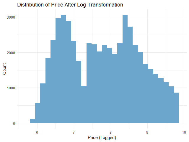
# Check the distribution of logged `price`
ggplot(dm,
       aes(x = price_log)) +
  
  ## Instantiate a histogram
  geom_histogram(fill = "skyblue3") +
  
  ## Add text elements
  labs(title = "Distribution of Price After Log Transformation",
       x = "Price (Logged)",
       y = "Count") +
  
  ## Set theme to minimal
  theme_minimal()

ผลลัพธ์:

จะเห็นได้ว่า การกระจายตัวของตัวแปรตามใกล้เคียงกับการกระจายตัวแบบปกติมากขึ้นแล้ว

🚄 Step 3. Split the Data

ในขั้นสุดท้ายก่อนใช้ linear regression เราจะแบ่งข้อมูลออกเป็น 2 ชุด:

Training set สำหรับสร้าง linear regression model
Test set สำหรับประเมินความสามารถของ linear regression model

ในบทความนี้ เราจะแบ่ง 80% ของ dataset เป็น training set และ 20% เป็น test set:

# Split the data

## Set seed for reproducibility
set.seed(181)

## Training index
train_index <- sample(nrow(dm),
                      0.8 * nrow(dm))

## Create training set
train_set <- dm[train_index, ]

## Create test set
test_set <- dm[-train_index, ]

ตอนนี้ เราพร้อมที่จะสร้าง linear regression model กันแล้ว

🏷️ Linear Regression Modelling

การสร้าง linear regression model มีอยู่ 3 ขั้นตอน ได้แก่:

Fit the model
Make predictions
Evaluate the model performance

💪 Step 1. Fit the Model

ในขั้นแรก เราจะสร้าง model ด้วย lm() ซึ่งต้องการ input 2 อย่าง:

lm(formula, data)

formula = สูตรการทำนาย โดยเราต้องกำหนดตัวแปรต้นและตัวแปรตาม
data = ชุดข้อมูลที่ใช้สร้าง model

ในการทำนายราคาเพชร เราจะใช้ lm() แบบนี้:

# Fit the model
linear_reg <- lm(price_log ~ .,
                 data = train_set)

อธิบาย code:

price_log ~ . หมายถึง ทำนายราคา (price_log) ด้วยตัวแปรต้นทั้งหมด (.)
data = train_set หมายถึง เรากำหนดชุดข้อมูลที่ใช้เป็น training set

เราสามารถดูข้อมูลของ model ได้ด้วย summary():

# View the model
summary(linear_reg)

ผลลัพธ์:

Call:
lm(formula = price_log ~ ., data = train_set)

Residuals:
    Min      1Q  Median      3Q     Max 
-2.2093 -0.0930  0.0019  0.0916  9.8935 

Coefficients: (1 not defined because of singularities)
                 Estimate Std. Error  t value Pr(>|t|)    
(Intercept)    -2.7959573  0.0705854  -39.611  < 2e-16 ***
carat          -0.5270039  0.0086582  -60.867  < 2e-16 ***
depth           0.0512357  0.0008077   63.437  < 2e-16 ***
table           0.0090154  0.0005249   17.175  < 2e-16 ***
x               1.1374016  0.0055578  204.651  < 2e-16 ***
y               0.0290584  0.0031345    9.271  < 2e-16 ***
z               0.0340298  0.0054896    6.199 5.73e-10 ***
cutFair        -0.1528658  0.0060005  -25.476  < 2e-16 ***
cutGood        -0.0639105  0.0036547  -17.487  < 2e-16 ***
`cutVery Good` -0.0313800  0.0025724  -12.199  < 2e-16 ***
cutPremium     -0.0451760  0.0026362  -17.137  < 2e-16 ***
cutIdeal               NA         NA       NA       NA    
colorE         -0.0573940  0.0032281  -17.779  < 2e-16 ***
colorF         -0.0892633  0.0032654  -27.336  < 2e-16 ***
colorG         -0.1573861  0.0032031  -49.136  < 2e-16 ***
colorH         -0.2592763  0.0034037  -76.175  < 2e-16 ***
colorI         -0.3864526  0.0038360 -100.742  < 2e-16 ***
colorJ         -0.5258789  0.0047183 -111.455  < 2e-16 ***
claritySI2      0.4431577  0.0079170   55.976  < 2e-16 ***
claritySI1      0.6087513  0.0078819   77.234  < 2e-16 ***
clarityVS2      0.7523161  0.0079211   94.976  < 2e-16 ***
clarityVS1      0.8200656  0.0080463  101.918  < 2e-16 ***
clarityVVS2     0.9381319  0.0082836  113.252  < 2e-16 ***
clarityVVS1     1.0033931  0.0085098  117.910  < 2e-16 ***
clarityIF       1.0898015  0.0092139  118.277  < 2e-16 ***
---
Signif. codes:  0 ‘***’ 0.001 ‘**’ 0.01 ‘*’ 0.05 ‘.’ 0.1 ‘ ’ 1

Residual standard error: 0.1825 on 43128 degrees of freedom
Multiple R-squared:  0.9677,	Adjusted R-squared:  0.9676 
F-statistic: 5.611e+04 on 23 and 43128 DF,  p-value: < 2.2e-16

Note: ดูวิธีการอ่านผลลัพธ์ได้ที่ Explaining the lm() Summary in R และ Understanding Linear Regression Output in R

🔮 Step 2. Make Predictions

ในขั้นที่สอง เราจะใช้ model เพื่อทำนายราคาด้วย predict():

# Predict in the outcome space
pred <- exp(pred_log)

# Preview predictions
head(pred_log)

ผลลัพธ์:

       2        5        9       16       19       22 
5.828071 5.816460 6.111859 5.777434 5.865820 6.088356

จะเห็นว่า ราคาที่ทำนายยังอยู่ในรูป log ซึ่งเราต้องแปลงกลับเป็นราคาปกติด้วย exp():

# Predict in the outcome space
pred <- exp(pred_log)

# Preview predictions
head(pred)

ผลลัพธ์:

       2        5        9       16       19       22 
339.7028 335.7812 451.1766 322.9295 352.7713 440.6961

เราสามารถเปรียบเทียบราคาจริงกับราคาที่ทำนาย พร้อมความคลาดเคลื่อน ได้ดังนี้:

# Compare predictions to actual
results <- data.frame(actual = round(exp(test_set$price_log), 2),
                      predicted = round(pred, 2),
                      diff = round(exp(test_set$price_log) - pred, 2))

# Print results
head(results)

ผลลัพธ์:

   actual predicted    diff
2     326    339.70  -13.70
5     335    335.78   -0.78
9     337    451.18 -114.18
16    345    322.93   22.07
19    351    352.77   -1.77
22    352    440.70  -88.70

🎯 Step 3. Evaluate the Model Performance

ในขั้นสุดท้าย เราจะประเมิน model โดยใช้ 2 ตัวชี้วัด ได้แก่:

Mean absolute error (MAE): ค่าเฉลี่ยความคลาดเคลื่อนโดยสัมบูรณ์
Root mean squared error (RMSE): ค่าเฉลี่ยความคลาดเคลื่อนแบบยกกำลังสอง

ทั้งสองตัวคำนวณความแตกต่างระหว่างสิ่งที่ทำนายและข้อมูลจริง ยิ่ง MAE และ RMSE สูง ก็หมายความว่า การทำนายมีความคาดเคลื่อนมาก แสดงว่า model ทำงานได้ไม่ดีนัก

ในทางกลับกัน ถ้า MAE และ RMSE น้อย ก็แสดงว่า การทำนายใกล้เคียงกับข้อมูลจริง และ model มีความแม่นยำสูง

(Note: เรียนรู้ความแตกต่างระหว่าง MAE และ RMSE ได้ที่ Loss Functions in Machine Learning Explained)

เราสามารถคำนวณ MAE และ RMSE ได้ดังนี้:

# Calculate MAE
mae <- mean(abs(results$diff))

# Calculate RMSE
rmse <- sqrt(mean((results$diff)^2))

# Print the results
cat("MAE:", round(mae, 2), "\n")
cat("RMSE:", round(rmse, 2))

ผลลัพธ์:

MAE: 491.71
RMSE: 1123.68

จากผลลัพธ์ เราจะเห็นว่า โดยเฉลี่ย model ทำนายราคาคลาดเคลื่อนไปประมาณ 492 ดอลล่าร์ (MAE)

😎 Summary

ในบทความนี้ เราได้ดูวิธีการทำ linear regression ในภาษา R กัน

เราดูวิธีการเตรียมข้อมูลสำหรับ linear regression:

One-hot encoding ด้วย model.matrix()
Log transformation ด้วย log()
Split data ด้วย sample()

สร้าง linear regression model ด้วย lm() พร้อมประเมิน model ด้วย predict() และการคำนวณค่า MAE และ RMSE

😺 GitHub

ดู code ทั้งหมดในบทความนี้ได้ที่ GitHub

📃 References

✅ R Book for Psychologists: หนังสือภาษา R สำหรับนักจิตวิทยา

📕 ขอฝากหนังสือเล่มแรกในชีวิตด้วยนะครับ 😆

Correlation
t-tests
ANOVA
Reliability
Factor analysis

แล้วทุกคนจะแปลกใจว่า ทำไมภาษา R ง่ายขนาดนี้ 🙂‍↕️

👉 สนใจดูรายละเอียดหนังสือได้ที่ meb:

ดูรายละเอียดหนังสือ R Book for Psychologists

2025-05-29

วิธีสร้าง Naïve Bayes classifier ใน 5 ขั้นตอนด้วย naivebayes package ในภาษา R – ตัวอย่างการทำนายประเภทดอกไม้ใน iris dataset
ในบทความนี้ เราจะมาทำความรู้กับ Naïve Bayes และดูวิธีสร้าง Naïve Bayes classifier ในภาษา R ด้วย naivebayes package กัน
👼 Naïve Bayes คืออะไร?

Naïve Bayes (NB) เป็น machine learning algorithm ประเภท supervised learning สำหรับทำนายกลุ่มของข้อมูล (classification)

NB ทำนายข้อมูล โดยวิเคราะห์ความน่าจะเป็นที่ 2 เหตุการณ์ (ตัวแปรต้นและตัวแปรตาม) จะเกิดขึ้นคู่กัน

ยกตัวอย่างเช่น การอนุมัติสินเชื่อ (อนุมัติ/ไม่อนุมัติ) ที่เกิดขึ้นอยู่กับ:
- รายได้: รายได้มาก -> อนุมัติ
- อายุ: อายุน้อย -> อนุมัติ
- ประวัติการขอสินเชื่อ: เคยขอแล้วผ่าน -> อนุมัติ
NB คำนวณความน่าจะเป็นของแต่ละปัจจัยต่อตัวแปรตาม (การอนุมัติ) โดยอนุมานว่า แต่ละปัจจัยเกิดแยกกัน (independent) แม้ว่าในความเป็นจริงหลายปัจจัยจะเกิดขึ้นร่วมกัน (dependent; เช่น อายุมาก -> รายได้มาก) ก็ตาม

เนื่องจาก NB มีการมองโลกอย่างง่าย จึงได้ชื่อว่า “naïve” หรือไร้เดียงนั่นเอง

แม้ว่า NB จะมีการมองโลกที่ไร้เดียงสา แต่ก็เป็น algorithm ที่:
1. เข้าใจได้ง่าย (เพราะไร้เดียงสา)
2. รวดเร็ว (เพราะใช้การวิเคราะห์อย่างง่าย)
3. น่าเชื่อถือ (มักจะทำนายได้แม่นยำ แม้จะมีมุมมองที่ไม่ตรงกับความเป็นจริง)
🧑‍💻 วิธีสร้าง NB Classifer ด้วย naivebayes Package

วิธีการสร้าง NB classifier ด้วย naivebayes package มี 5 ขั้นตอน ได้แก่:
1. Install and load the package
2. Load and preview the dataset
3. Split the dataset
4. Create a NB model
5. Evaluate the model
.

1️⃣ Step 1. Install & Load the Package

ในขั้นแรก เราต้องติดตั้งและเรียกใช้งาน naivebayes package:
```
# Install and load the package
## Install
install.packages("naivebayes")
## Load
library(naivebayes)
```
Note: เราทำการติดตั้งแค่ครั้งแรกครั้งเดียว แต่การเรียกใช้ต้องทำทุกครั้งทุกเริ่ม session ใหม่

.

2️⃣ Step 2. Load & Preview the Dataset

ในขั้นที่สอง ให้เราโหลด dataset ที่จะใช้งาน

โดยในบทความนี้ เราจะใช้ built-in dataset ในภาษา R ชื่อ iris dataset

iris dataset มีกลีบดอกของข้อมูลดอกไม้ 3 ชนิด ได้แก่:
- Iris setosa
- Iris virginica
- Iris versicolor
เป้าหมายของเรา คือ ทำนายประเภทของดอกไม้จากความกว้างและความยาวกลีบดอก

เนื่องจากเป็น built-in dataset เราสามารถโหลด iris dataset ด้วยคำสั่ง data():
```
# Load
data(iris)
```
จากนั้น เราสามารถใช้คำสั่ง head() เพื่อ preview ข้อมูล:
```
# Preview
head(iris)
```
ผลลัพธ์:
```
  Sepal.Length Sepal.Width Petal.Length Petal.Width Species
1          5.1         3.5          1.4         0.2  setosa
2          4.9         3.0          1.4         0.2  setosa
3          4.7         3.2          1.3         0.2  setosa
4          4.6         3.1          1.5         0.2  setosa
5          5.0         3.6          1.4         0.2  setosa
6          5.4         3.9          1.7         0.4  setosa
```
Note: จะเห็นว่า iris dataset มีข้อมูลทั้งหมด 5 columns คือ ความยาวและความกว้างของกลีบดอกชั้นนอก (sepal) และความยาวและความกว้างของกลีบดอกชั้นใน (petal) รวมทั้งประเภทดอกไม้ (species)

เนื่องจาก NB classifier ต้องการตัวแปรตามที่เป็น factor เราต้องเช็กได้ว่า Species เป็น data type ไหนด้วยคำสั่ง str():
```
# Preview
str(iris)
```
ผลลัพธ์:
```
'data.frame':	150 obs. of  5 variables:
 $ Sepal.Length: num  5.1 4.9 4.7 4.6 5 5.4 4.6 5 4.4 4.9 ...
 $ Sepal.Width : num  3.5 3 3.2 3.1 3.6 3.9 3.4 3.4 2.9 3.1 ...
 $ Petal.Length: num  1.4 1.4 1.3 1.5 1.4 1.7 1.4 1.5 1.4 1.5 ...
 $ Petal.Width : num  0.2 0.2 0.2 0.2 0.2 0.4 0.3 0.2 0.2 0.1 ...
 $ Species     : Factor w/ 3 levels "setosa","versicolor",..: 1 1 1 1 1 1 1 1 1 1 ...
```
จะเห็นได้ว่า Species เป็น factor อยู่แล้ว และพร้อมที่ใช้สร้าง NB classifier

.

3️⃣ Step 3. Split the Dataset

ในขั้นที่สาม เราจะแบ่งข้อมูลเป็น 2 ชุด:
1. Training set เพื่อสร้าง NB classifier
2. Test set เพื่อทดสอบประสิทธิภาพของ NB classifier
ขั้นแรกในการแบ่งข้อมูล ให้เราสุ่มเลือก row index ที่จะอยู่ใน training set:
```
# Set seed for reproducibility
set.seed(2025)
# Create a training index
training_index <- sample(1:nrow(iris),
                         0.7 * nrow(iris))
```
จากนั้น ใช้ row index ที่ได้แบ่งข้อมูลเป็น 2 ชุด:
```
# Split the dataset
train_set <- iris[training_index, ]
test_set <- iris[-training_index, ]
```
.

4️⃣ Step 4. Create a NB Model

ในขั้นที่สี่ เราจะสร้าง NB classifier โดยใช้ naive_bayes() จาก naivebayes package

naive_bayes() ต้องการ input 2 อย่าง:
1. Formula: ตัวแปรต้นและตัวแปรตามที่ต้องการใช้สร้าง model โดยในกรณีนี้ คือ ทำนาย Species ด้วยข้อมูลที่เหลือทั้งหมด (.)
2. Data: dataset ที่จะใช้สร้าง model ซึ่งในกรณีนี้ คือ train_set
```
# Create a NB model
nb <- naive_bayes(Species ~ .,
                  data = train_set)
```
เมื่อเราได้ NB classifier มาแล้ว เรามาลองใช้ model ทำนายประเภทดอกไม้กัน:
```
# Predict the outcomes
pred <- predict(nb,
                newdata = test_set[, 1:4],
                type = "class")
print(pred)
```
ผลลัพธ์:
```
 [1] setosa     setosa     setosa     setosa     setosa    
 [6] setosa     setosa     setosa     setosa     setosa    
[11] setosa     setosa     setosa     setosa     setosa    
[16] virginica  versicolor versicolor versicolor versicolor
[21] virginica  versicolor versicolor versicolor versicolor
[26] versicolor virginica  versicolor versicolor versicolor
[31] versicolor versicolor versicolor versicolor virginica 
[36] virginica  virginica  virginica  virginica  virginica 
[41] virginica  virginica  virginica  virginica  virginica 
Levels: setosa versicolor virginica
```
.

5️⃣ Step 5. Evaluate the Model

ในขั้นสุดท้าย เราจะประเมินประสิทธิภาพของ model ด้วยการคำนวณ accuracy หรือ สัดส่วนของคำตอบที่ model ตอบถูก:

Accuracy = Correct predictions / Total predictions

เราสามารถหาค่า accuracy ได้โดยเริ่มสร้าง confusion matrix ก่อน:
```
# Create a confusion matrix
cm <- table(Predicted = pred, 
            Actual = test_set$Species)
print(cm)
```
ผลลัพธ์:
```
            Actual
Predicted    setosa versicolor virginica
  setosa         15          0         0
  versicolor      0         16         0
  virginica       0          3        11
```
จากนั้น นำจำนวนคำตอบที่ถูกต้องและจำนวนคำตอบทั้งหมดมาหาค่า accuracy:
```
# Calculate the accuracy
accuracy <- sum(diag(cm)) / sum(cm)
cat("Accuracy:", round(accuracy, 2))
```
ผลลัพธ์:
```
Accuracy: 0.93
```
จะเห็นได้ว่า NB classifier ที่เป็น model ไร้เดียงสาของเรา มีความแม่นยำในการทำนายสูงถึง 93%

😺 GitHub

ดู code ทั้งหมดในบทความนี้ได้ที่ GitHub

📃 References
✅ R Book for Psychologists: หนังสือภาษา R สำหรับนักจิตวิทยา

📕 ขอฝากหนังสือเล่มแรกในชีวิตด้วยนะครับ 😆

🙋 ใครที่กำลังเรียนจิตวิทยาหรือทำงานสายจิตวิทยา และเบื่อที่ต้องใช้ software ราคาแพงอย่าง SPSS และ Excel เพื่อทำข้อมูล

💪 ผมขอแนะนำ R Book for Psychologists หนังสือสอนใช้ภาษา R เพื่อการวิเคราะห์ข้อมูลทางจิตวิทยา ที่เขียนมาเพื่อนักจิตวิทยาที่ไม่เคยมีประสบการณ์เขียน code มาก่อน

ในหนังสือ เราจะปูพื้นฐานภาษา R และพาไปดูวิธีวิเคราะห์สถิติที่ใช้บ่อยกัน เช่น:
- Correlation
- t-tests
- ANOVA
- Reliability
- Factor analysis
🚀 เมื่ออ่านและทำตามตัวอย่างใน R Book for Psychologists ทุกคนจะไม่ต้องพึง SPSS และ Excel ในการทำงานอีกต่อไป และสามารถวิเคราะห์ข้อมูลด้วยตัวเองได้ด้วยความมั่นใจ

แล้วทุกคนจะแปลกใจว่า ทำไมภาษา R ง่ายขนาดนี้ 🙂‍↕️

👉 สนใจดูรายละเอียดหนังสือได้ที่ meb:

ดูรายละเอียดหนังสือ R Book for Psychologists
Share this:
X
Facebook
Like Loading…
2025-04-10
วิธีสร้าง KNN model ใน 5 ขั้นตอนด้วย class package ในภาษา R – ตัวอย่างการทำนายประเภทดอกไม้ใน iris dataset
ในบทความนี้ เราจะมาทำความรู้กันกับ KNN model และวิธีสร้าง KNN model ด้วย class package ในภาษา R กัน
KNN หรือ K-Nearest Neighbors เป็น machine learning algorithm ประเภท supervised learning ซึ่งใช้ได้กับงานประเภท classification (จัดกลุ่ม) และ regression (ทำนายแนวโน้ม)

การทำงานของ KNN ตรงไปตรงมา คือ ทำนายข้อมูลโดยการดูจากข้อมูลใกล้เคียง จำนวน k ข้อมูล (เราสามารถกำหนดค่า k เองได้)

ยกตัวอย่างเช่น เราต้องการใช้ KNN ทำนายราคาหุ้น KNN จะดูราคาหุ้นที่อยู่ใกล้เคียงกับหุ้นที่เราต้องการทำนายราคา เช่น 5 หุ้นใกล้เคียง โดย:
- 2/5 หุ้น = ราคาลง
- 3/5 หุ้น = ราคาขึ้น
KNN จะทำนายว่า หุ้นในใจของเรา จะราคาขึ้น เพราะหุ้นใกล้เคียงส่วนใหญ่ปรับราคาขึ้น เป็นต้น

💻 KNN in R With class Package

เราสามารถสร้าง KNN model ในภาษา R ด้วย class package โดยมี 5 ขั้นตอนดังนี้:
1. Get class package
2. Load the dataset
3. Prepare the data
4. Train a KNN model
5. Evaluate the model
เราไปดูตัวอย่างการสร้าง KNN model เพื่อทำนายประเภทดอกไม้ ด้วย iris dataset กัน

1️⃣ Step 1. Get class Package

ในขั้นแรก ให้เราติดตั้งและเรียกใช้งาน class package

ติดตั้ง (ทำครั้งเดียว):
```
# Install
install.packages("class")
```
เรียกใช้งาน (ทำทุกครั้งที่เริ่ม session ใหม่):
```
# Load
library(class)
```
2️⃣ Step 2. Get the Dataset

ในขั้นที่สอง ให้เราโหลด dataset ที่จะใช้งาน

โดยในบทความนี้ เราจะใช้ iris ที่มีข้อมูลดอกไม้ 3 ชนิด ได้แก่:
- Iris setosa
- Iris virginica
- Iris versicolor
นอกจากประเภทดอกไม้ (species) iris dataset ยังประกอบด้วยความกว้าง (width) และความยาว (length) ของกลีบดอกชั้นนอก (sepal) และชั้นใน (petal)

เนื่องจาก iris เป็น built-in dataset ใน ภาษา R เราสามารถโหลดข้อมูลด้วยคำสั่ง data() ได้:
```
# Load
data(iris)
```
เมื่อโหลดแล้ว เราสามารถดูตัวอย่าง dataset ได้ด้วย head():
```
# Preview
head(iris)
```
ผลลัพธ์:
```
  Sepal.Length Sepal.Width Petal.Length Petal.Width Species
1          5.1         3.5          1.4         0.2  setosa
2          4.9         3.0          1.4         0.2  setosa
3          4.7         3.2          1.3         0.2  setosa
4          4.6         3.1          1.5         0.2  setosa
5          5.0         3.6          1.4         0.2  setosa
6          5.4         3.9          1.7         0.4  setosa
```
3️⃣ Step 3. Prepare Data

ในขั้นที่สาม เราจะเตรียมข้อมูล เพื่อใช้สร้าง KNN model

โดยสำหรับ iris dataset เราจะทำ 3 อย่าง คือ:
1. Normalise data
2. Split data
3. Separate features from the label
.

📉 Normalise Data

เนื่องจาก KNN model อ้างอิงระยะห่างระหว่างข้อมูลในการทำนายผลลัพธ์ ข้อมูลที่มีช่วงกว้าง (เช่น 0-100) จะมีน้ำหนักกว่าข้อมูลที่มีช่วงแคบ (เช่น 0-10) และทำให้ model ของเรา bias ได้

เพื่อป้องกันความเสี่ยงนี้ เราต้อง normalise ข้อมูล หรือการทำให้ข้อมูลมีช่วงมีช่วงข้อมูลเดียวกัน

การทำ normalisation มีหลายวิธี แต่วิธีที่นิยมใช้กับ KNN คือ min-max normalisation ซึ่งเปลี่ยนช่วงข้อมูลให้อยู่ในช่วง 0-1 ผ่านสูตร:
```
(X - Min) / (Max - Min)
```
- X คือ ข้อมูล
- Min คือ ค่าที่น้อยที่สุด
- Max คือ ค่าที่มากที่สุด
ในภาษา R เราไม่มี function ที่ใช้ทำ min-max normalisation ได้โดยตรง เราเลยต้องเขียน function ขึ้นมาใช้เอง:
```
# Define a function for normalisation
normalise <- function(x) {
  return((x - min(x)) / (max(x) - min(x)))
}
```
จากนั้น ให้เราใช้ function นี้กับ columns ที่เป็นตัวเลข (numeric) เช่น Sepal.Length แล้วเก็บผลลัพธ์ไว้ใน data frame ใหม่ ชื่อ iris_normalises:
```
# Apply the function to the dataset
iris_normalised <- as.data.frame(lapply(iris[, 1:4],
                                        normalise))
```
เนื่องจากตอนที่เราใช้ function เราตัด column ที่ไม่ใช่ตัวเลขออก ทำให้ iris_normalised ไม่มี column Species

เราสามารถใส่ Species กลับเข้าไป เพื่อใช้ในขั้นตอนถัดไป แบบนี้:
```
# Add species column back into the data frame
iris_normalised$Species <- iris$Species
```
สุดท้าย เราเช็กผลลัพธ์ด้วยการเรียกดูสถิติของ iris_normalised:
```
# Check the results
summary(iris_normalised)
```
ผลลัพธ์:
```
  Sepal.Length     Sepal.Width    
 Min.   :0.0000   Min.   :0.0000  
 1st Qu.:0.2222   1st Qu.:0.3333  
 Median :0.4167   Median :0.4167  
 Mean   :0.4287   Mean   :0.4406  
 3rd Qu.:0.5833   3rd Qu.:0.5417  
 Max.   :1.0000   Max.   :1.0000  
  Petal.Length     Petal.Width     
 Min.   :0.0000   Min.   :0.00000  
 1st Qu.:0.1017   1st Qu.:0.08333  
 Median :0.5678   Median :0.50000  
 Mean   :0.4675   Mean   :0.45806  
 3rd Qu.:0.6949   3rd Qu.:0.70833  
 Max.   :1.0000   Max.   :1.00000  
       Species  
 setosa    :50  
 versicolor:50  
 virginica :50  
```
จะเห็นว่า:
1. Columns ที่เป็นตัวเลข มีช่วงอยู่ระหว่าง 0 และ 1
2. เรายังมี column Species อยู่
.

🪓 Split Data

ในการสร้าง KNN model เราควรแบ่ง dataset ที่มีเป็น 2 ส่วน คือ:
1. Training set: ใช้สำหรับสร้าง model
2. Test set: ใช้สำหรับประเมิน model
เราเริ่มแบ่งข้อมูลด้วยการสุ่ม row index ที่จะอยู่ใน training set:
```
# Set seed for reproducibility
set.seed(2025)

# Create a training index
train_index <- sample(1:nrow(iris_normalised),
                      0.7 * nrow(iris_normalised))
```
จากนั้น subset ข้อมูลด้วย row index ที่สุ่มไว้:
```
# Split the data
train_set <- iris_normalised[train_index, ]
test_set <- iris_normalised[-train_index, ]
```
.

🏷️ Separate Features From Label

ขั้นตอนสุดท้ายในการเตรียมข้อมูล คือ แยก features หรือ X (columns ที่จะใช้ทำนาย) ออกจาก label หรือ Y (สิ่งที่ต้องการทำนาย):
```
# Separate features from label

## Training set
train_X <- train_set[, 1:4]
train_Y <- train_set$Species

## Test set
test_X <- test_set[, 1:4]
test_Y <- test_set$Species
```
4️⃣ Step 4. Train a KNN Model

ขั้นที่สี่เป็นขั้นที่เราสร้าง KNN model ขึ้นมา โดยเรียกใช้ knn() จาก class package

ทั้งนี้ knn() ต้องการ input 3 อย่าง:
1. train: fatures จาก training set
2. test: feature จาก test set
3. cl: label จาก training set
4. k: จำนวนข้อมูลใกล้เคียงที่จะใช้ทำนายผลลัพธ์
```
# Train a KNN model
pred <- knn(train = train_X,
            test = test_X,
            cl = train_Y,
            k = 5)
```
ในตัวอย่าง เรากำหนด k = 5 เพื่อทำนายผลลัพธ์โดยดูจากข้อมูลที่ใกล้เคียง 5 อันดับแรก

5️⃣ Step 5. Evaluate the Model

หลังจากได้ model แล้ว เราประเมินประสิทธิภาพของ model ในการทำนายผลลัพธ์ ซึ่งเราทำได้ง่าย ๆ โดยคำนวณ accuracy หรือสัดส่วนของข้อมูลที่ model ตอบถูกต่อจำนวนข้อมูลทั้งหมด:
```
Accuracy = Correct predictions / Total predictions
```
ในภาษา R ให้เราสร้าง confusion matrix หรือ matrix แสดงจำนวนคำตอบที่ถูกและผิด ด้วย table() function:
```
# Create a confusion matrix
cm <- table(Predicted = predictions,
            Actual = test_Y)

# Print the matrix
print(cm)
```
ผลลัพธ์:
```
            Actual
Predicted    setosa versicolor virginica
  setosa         15          0         0
  versicolor      0         17         0
  virginica       0          2        11
```
Note: จะเห็นได้ว่า model เราตอบถูกเป็นส่วนใหญ่ (ราว 90%)

จากนั้น คำนวณ accuracy ด้วย sum() และ diag():
```
# Calculate accuracy
acc <- sum(diag(cm)) / sum(cm)

# Print accuracy
cat("Accuracy:", round(acc, 2))
```
ผลลัพธ์:
```
Accuracy: 0.96
```
จากผลลัพธ์ เราจะเห็นว่า model มีความแม่นยำสูงถึง 96%

🍩 Bonus: Fine-Tuning

ในบางครั้ง ค่า k ที่เราตั้งไว้ อาจไม่ได้ทำให้เราได้ KNN model ที่ดีที่สุด

แทนที่เราจะแทนค่า k ใหม่ไปเรื่อย ๆ เราสามารถใช้ for loop เพื่อหาค่า k ที่ทำให้เราได้ model ที่ดีที่สุดได้

ให้เราเริ่มจากสร้าง vector ที่มีค่า k ที่ต้องการ:
```
# Create a set of k values
k_values <- 1:20
```
และ vector สำหรับเก็บค่า accuracy ของค่า k แต่ละตัว:
```
# Createa a vector for accuracy results
accuracy_results <- numeric(length(k_values))
```
แล้วใช้ for loop เพื่อหาค่า accuracy ของค่า k:
```
# For-loop through the k values
for (i in seq_along(k_values)) {
  
  ## Set the k value
  k <- k_values[i]
  
  ## Create a KNN model
  predictions <- knn(train = train_X,
                     test = test_X,
                     cl = train_Y,
                     k = k)
  
  ## Create a confusion matrix
  cm <- table(Predicted = predictions,
              Actual = test_Y)
  
  ## Calculate accuracy
  accuracy_results[i] <- sum(diag(cm)) / sum(cm)
}

# Find the best k and the corresponding accuracy
best_k <- k_values[which.max(accuracy_results)]
best_accuracy <- max(accuracy_results)

# Print best k and accuracy
cat(paste("Best k:", best_k),
    paste("Accuracy:", round(best_accuracy, 2)),
    sep = "\n")
```
ผลลัพธ์:
```
Best k: 12
Accuracy: 0.98
```
แสดงว่า ค่า k ที่ดีที่สุด คือ 12 โดยมี accuracy เท่ากับ 98%

นอกจากนี้ เรายังสามารถสร้างกราฟ เพื่อช่วยทำความเข้าใจผลของค่า k ต่อ accuracy:
```
# Plot the results
plot(k_values,
     accuracy_results,
     type = "b",
     pch = 19,
     col = "blue",
     xlab = "Number of Neighbors (k)",
     ylab = "Accuracy",
     main = "KNN Model Accuracy for Different k Values")
grid()
```
ผลลัพธ์:

จะเห็นได้ว่า k = 12 ให้ accuracy ที่ดีที่สุด และ k = 20 ให้ accuracy ต่ำที่สุด ส่วนค่า k อื่น ๆ ให้ accuracy ในช่วง 93 ถึง 96%

😺 GitHub

ดู code ทั้งหมดในบทความนี้ได้ที่ GitHub

📃 References
✅ R Book for Psychologists: หนังสือภาษา R สำหรับนักจิตวิทยา

📕 ขอฝากหนังสือเล่มแรกในชีวิตด้วยนะครับ 😆

🙋 ใครที่กำลังเรียนจิตวิทยาหรือทำงานสายจิตวิทยา และเบื่อที่ต้องใช้ software ราคาแพงอย่าง SPSS และ Excel เพื่อทำข้อมูล

💪 ผมขอแนะนำ R Book for Psychologists หนังสือสอนใช้ภาษา R เพื่อการวิเคราะห์ข้อมูลทางจิตวิทยา ที่เขียนมาเพื่อนักจิตวิทยาที่ไม่เคยมีประสบการณ์เขียน code มาก่อน

ในหนังสือ เราจะปูพื้นฐานภาษา R และพาไปดูวิธีวิเคราะห์สถิติที่ใช้บ่อยกัน เช่น:
- Correlation
- t-tests
- ANOVA
- Reliability
- Factor analysis
🚀 เมื่ออ่านและทำตามตัวอย่างใน R Book for Psychologists ทุกคนจะไม่ต้องพึง SPSS และ Excel ในการทำงานอีกต่อไป และสามารถวิเคราะห์ข้อมูลด้วยตัวเองได้ด้วยความมั่นใจ

แล้วทุกคนจะแปลกใจว่า ทำไมภาษา R ง่ายขนาดนี้ 🙂‍↕️

👉 สนใจดูรายละเอียดหนังสือได้ที่ meb:

ดูรายละเอียดหนังสือ R Book for Psychologists
Share this:
X
Facebook
Like Loading…
2025-04-03
แนะนำ dtplyr: package เชื่อม dplyr และ data.table เพื่อการทำ data wrangling กับข้อมูลขนาดใหญ่ที่ง่ายและรวดเร็ว — ตัวอย่างจาก mtcars dataset
ในบทความนี้ เรามาความรู้จักกับ package ในภาษา R ที่เรียกว่า dtplyr กัน
🏎️ dtplyr คืออะไร?

dtplyr เป็น package ที่เชื่อม 2 libraries ยอดนิยมสำหรับ data wrangling เข้าด้วยกัน ได้แก่:

.

Library #1. dplyr ซี่งมี verb-based syntax ที่ใช้งานง่าย

เช่น จาก mtcars dataset เลือกรถเกียร์ manual (am == 1) ที่มี miles/gallon (mpg) ตั้งแต่ 20 ขึ้นไป โดยเรียงจากมากไปน้อย:
```
# dplyr
mtcars |>
  filter(am == 1 & mpg >= 20) |>
  select(model, mpg) |>
  arrange(desc(mpg))
```
Note: mtcars ถูกปรับให้มี column ชื่อ model (ดู code ในการเพิ่ม column ได้ใน GitHub)

.

Library #2. data.table ซึ่งมี syntax ที่เข้าใจยากกว่า:
```
# data.table
mtcars_dt[am == 1 & mpg >= 20, .(model, mpg)][order(-mpg)]
```
Note: mtcars_dt เป็น dataset ที่ถูกเปลี่ยนจาก data.frame เป็น data.table object เพื่อใช้งานกับ data.table

แต่มีจุดเด่น คือ ประมวลผลได้เร็ว เหมาะกับการทำงานกับ data ขนาดใหญ่

.

dtplyr เชื่อม dplyr เข้ากับ data.table โดยการแปล dplyr syntax ให้เป็น data.table syntax ทำให้เราทำงานได้ง่ายและรวดเร็ว

🧑‍💻 วิธีใช้ dytplyr

เราสามารถใช้ dtplyr ได้ใน 3 ขั้นตอนง่าย ๆ:
1. Install and load dtplyr
2. Create a lazy data.table
3. Execute the syntax
.

1️⃣ ขั้นที่ 1. Install & Load dtplyr

ในการใช้งาน dtplyr เราต้องเรียกใช้ dplyr ด้วยเสมอ

ดังนั้น ในการติดตั้ง เราต้องติดตั้งทั้ง dtplyr และ dplyr:
```
# Install
install.packages("dplyr")
install.packages("dtplyr")
```
เมื่อติดตั้งแล้ว ให้เราเรียกใช้งาน dtplyr และ dplyr ทุกครั้งที่เริ่ม session ในการทำงาน:
```
# Load
library(dplyr)
library(dtplyr)
```
Note: คู่มือการใช้ dtplyr แนะนำให้โหลด data.table ด้วย เพื่อใช้ functions ของ data.table ในการทำงาน

.

2️⃣ ขั้นที่ 2. Create a Lazy data.table

หลังเรียกใช้งาน dtplyr ให้เราสร้าง dataset ที่เป็น lazy data.table object ขึ้นมา เพื่อช่วยให้ dtplyr เปลี่ยนคำสั่งของ dplyr เป็นคำสั่งของ data.table ได้:
```
# Convert mtcars dataset into lazy data.table object
mtcars_ldt <- lazy_dt(mtcars)
```
.

3️⃣ ขั้นที่ 3. Execute the Syntax

ในขั้นสุดท้าย เราสามารถเริ่มทำงานโดยใช้ syntax ของ dplyr ได้เลย:
```
# Execute the syntax
mtcars_ldt |>
  filter(am == 1 & mpg >= 20) |>
  select(model, mpg) |>
  arrange(desc(mpg)) |>
  as.data.table()
```
ผลลัพธ์:
```
             model   mpg
            <char> <num>
 1: Toyota Corolla  33.9
 2:       Fiat 128  32.4
 3:    Honda Civic  30.4
 4:   Lotus Europa  30.4
 5:      Fiat X1-9  27.3
 6:  Porsche 914-2  26.0
 7:     Datsun 710  22.8
 8:     Volvo 142E  21.4
 9:      Mazda RX4  21.0
10:  Mazda RX4 Wag  21.0
```
จะสังเกตว่า ใน code บรรทัดสุดท้าย เราเพิ่ม as.data.table() เข้ามาเพื่อบอกให้ dtplyr รู้ว่า เราเขียน syntax เสร็จแล้ว และพร้อมให้แปลงให้เป็น data.table syntax

ทั้งนี้ ถ้าเราเขียนโดยไม่มี as.data.table():
```
# Execute the syntax, without as.data.table()
mtcars_ldt |>
  filter(am == 1 & mpg >= 20) |>
  select(model, mpg) |>
  arrange(desc(mpg))
```
เราจะได้ผลลัพธ์ที่เป็นแค่ preview ที่ไม่สามารถนำไปใช้งานต่อได้:
```
  model            mpg
  <chr>          <dbl>
1 Toyota Corolla  33.9
2 Fiat 128        32.4
3 Honda Civic     30.4
4 Lotus Europa    30.4
5 Fiat X1-9       27.3
6 Porsche 914-2   26  
# ℹ 4 more rows
# ℹ Use `print(n = ...)` to see more rows
```
ดังนั้น ถ้าเราต้องการผลลัพธ์ทั้งหมด เราต้องใช้ as.data.table() ในการรันคำสั่งทุกครั้ง

Note: เราสามารถใช้คำสั่งอื่น ๆ แทน as.data.table() ได้ โดยจะให้ผลลัพธ์ที่แตกต่างกันไปดังนี้:

Function ผลลัพธ์ที่ส่งกลับมา
as.data.table() data.table
as.data.frame() data.frame
as.tibble() tibble
collect() tibble
pull() Single column

😺 GitHub

ดู code ทั้งหมดในบทความนี้ได้ที่ GitHub

📃 References
✅ R Book for Psychologists: หนังสือภาษา R สำหรับนักจิตวิทยา

📕 ขอฝากหนังสือเล่มแรกในชีวิตด้วยนะครับ 😆

🙋 ใครที่กำลังเรียนจิตวิทยาหรือทำงานสายจิตวิทยา และเบื่อที่ต้องใช้ software ราคาแพงอย่าง SPSS และ Excel เพื่อทำข้อมูล

💪 ผมขอแนะนำ R Book for Psychologists หนังสือสอนใช้ภาษา R เพื่อการวิเคราะห์ข้อมูลทางจิตวิทยา ที่เขียนมาเพื่อนักจิตวิทยาที่ไม่เคยมีประสบการณ์เขียน code มาก่อน

ในหนังสือ เราจะปูพื้นฐานภาษา R และพาไปดูวิธีวิเคราะห์สถิติที่ใช้บ่อยกัน เช่น:
- Correlation
- t-tests
- ANOVA
- Reliability
- Factor analysis
🚀 เมื่ออ่านและทำตามตัวอย่างใน R Book for Psychologists ทุกคนจะไม่ต้องพึง SPSS และ Excel ในการทำงานอีกต่อไป และสามารถวิเคราะห์ข้อมูลด้วยตัวเองได้ด้วยความมั่นใจ

แล้วทุกคนจะแปลกใจว่า ทำไมภาษา R ง่ายขนาดนี้ 🙂‍↕️

👉 สนใจดูรายละเอียดหนังสือได้ที่ meb:

ดูรายละเอียดหนังสือ R Book for Psychologists
Share this:
X
Facebook
Like Loading…
2025-03-06

Function	ผลลัพธ์ที่ส่งกลับมา
`as.data.table()`	`data.table`
`as.data.frame()`	`data.frame`
`as.tibble()`	`tibble`
`collect()`	`tibble`
`pull()`	Single column

Tag: R programming

1️⃣ Creating

2️⃣ Previewing

👀 View()

🙊 head()

🐒 tail()

🏗️ str()

🧮 summary()

💠 dim()

🚣 nrow()

🏦 ncol()

3️⃣ Indexing

💰 Using $

🔳 Using [[]]

4️⃣ Subsetting

🍽️ df[rows, cols]

🔪 subset()

5️⃣ Filtering

🍽️ df[rows, cols]

🔪 subset()

6️⃣ Sorting

⬇️ Ascending

⬆️ Descending

↔️ Sort by Multiple Columns

7️⃣ Aggregating

8️⃣ Adding Columns

9️⃣ Removing Columns

🔟 Binding

🤝 rbind()

🤲 cbind()

😺 GitHub

📃 References

✅ R Book for Psychologists: หนังสือภาษา R สำหรับนักจิตวิทยา

Share this:

Share this:

🏁 Getting Started

1️⃣ Install & Load Packages

2️⃣ Load Dataset

🔄️ Converting

1️⃣ การแปลงข้อมูลให้เป็น Datetime

2️⃣ การแปลงข้อมูลให้เป็น Time Series

🤷‍♂️ Missing Values

📈 Plotting

✂️ Subsetting

1️⃣ window()

2️⃣ Boolean Masking

3️⃣ Specific Date

🧮 Aggregating

🪟 Rolling Window

1️⃣ roll*()

2️⃣ rollapply()

➡️ Expanding Window

😎 Summary

😺 View Code in GitHub

📃 References

✅ R Book for Psychologists: หนังสือภาษา R สำหรับนักจิตวิทยา

Share this:

🚀 XGBoost คืออะไร?

💻 XGBoost ในภาษา R

1️⃣ Install & Load the Package

2️⃣ Load & Prepare the Data

3️⃣ Split the Data

4️⃣ Train the Model

5️⃣ Evaluate the Model

💪 Summary

😺 GitHub

📃 References

✅ R Book for Psychologists: หนังสือภาษา R สำหรับนักจิตวิทยา

Share this:

🤔 GLM คืออะไร?

💻 GLM ในภาษา R

☕ ตัวอย่างข้อมูล: coffee_shop

1️⃣ Linear Regression

2️⃣ Logistic Regression

3️⃣ Poisson Regression

💪 Summary

😺 GitHub

📃 References

✅ R Book for Psychologists: หนังสือภาษา R สำหรับนักจิตวิทยา

Share this:

**1️⃣ roll*()**