Tag: Machine learning

  • Machine Learning in R: รวบรวม 13 บทความสอนสร้าง Machine Learning ในภาษา R

    Machine Learning in R: รวบรวม 13 บทความสอนสร้าง Machine Learning ในภาษา R

    ภาษา R มี packages จำนวนมาก สำหรับสร้าง machine learning models

    ในบทความนี้ ผมรวบรวม 13 บทความสอนทำ machine learning ซึ่งแบ่งได้เป็น 4 กลุ่ม ดังนี้:

    1. Supervised learning models หรือการ train models แบบมีเฉลย
    2. Tree-based models หรือการสร้าง model ที่ใช้ decision trees
    3. Unsupervised learning models หรือการ train models แบบไม่มีเฉลย
    4. All-in-one packages หรือ packages สำหรับทำ machine learning แบบครบครัน ตั้งแต่การเตรียมข้อมูลไปจนถึงการประเมินประสิทธิภาพ รวมทั้งใช้ model ได้ตามต้องการ

    กลุ่มที่ 1. Supervised learning models (4 บทความ):

    1. KNN
    2. Naïve Bayes
    3. Linear regression
    4. Logistic regression
    5. Generalised linear models

    กลุ่มที่ 2. Tree-based models (3 บทความ):

    1. ภาค 1: Single tree และ random forest 1
    2. ภาค 2: Random forest 2
    3. ภาค 3: Boosted trees

    กลุ่มที่ 3. Unsupervised learning models (3 บทความ):

    1. k-means
    2. Hierarchical clustering analysis (HCA)
    3. Principal component analysis (PCA)

    กลุ่มที่ 4. All-in-one packages (2 บทความ):

    1. caret (เป็น package ที่เก่ากว่า)
    2. tidymodels (เป็น package ที่ใหม่กว่า)
  • สอนปลูกต้นไม้ในภาษา R (ภาค 3): 5 ขั้นตอนการสร้าง Boosted Trees ด้วย xgboost package ในภาษา R — ตัวอย่างการทำนายระดับการกินน้ำมันของรถใน mpg dataset

    สอนปลูกต้นไม้ในภาษา R (ภาค 3): 5 ขั้นตอนการสร้าง Boosted Trees ด้วย xgboost package ในภาษา R — ตัวอย่างการทำนายระดับการกินน้ำมันของรถใน mpg dataset

    ในบทความนี้ เราจะไปทำความรู้จักกับ eXtreme Gradient Boosting (XGBoost) และวิธีสร้าง XGBoost model ในภาษา R ด้วย xgboost package กัน

    ถ้าพร้อมแล้ว ไปเริ่มกันเลย


    1. 🚀 XGBoost คืออะไร?
    2. 💻 XGBoost ในภาษา R
    3. 1️⃣ Install & Load the Package
    4. 2️⃣ Load & Prepare the Data
    5. 3️⃣ Split the Data
    6. 4️⃣ Train the Model
    7. 5️⃣ Evaluate the Model
    8. 💪 Summary
    9. 😺 GitHub
    10. 📃 References
    11. ✅ R Book for Psychologists: หนังสือภาษา R สำหรับนักจิตวิทยา

    อ่านเกี่ยวกับการปลูกต้นไม้ในภาษา R ภาคก่อน ๆ ได้ที่:


    🚀 XGBoost คืออะไร?

    XGBoost เป็น machine learning model ที่จัดอยู่ในกลุ่ม tree-based models หรือ models ที่ทำนายข้อมูลด้วย decision tree อย่าง single decision tree และ random forest

    ใน XGBoost, decision trees จะถูกสร้างขึ้นมาเป็นรอบ ๆ โดยในแต่ละรอบ decision trees ใหม่จะเรียนรู้จากความผิดพลาดของรอบก่อน ซึ่งจะทำให้ decision trees ใหม่มีความสามารถที่ดีขึ้นเรื่อย ๆ

    เมื่อสิ้นสุดการสร้าง XGBoost ใช้ผลรวมของ decision trees ทุกต้นในการทำนายข้อมูล ดังนี้:

    • Regression problem: หาค่าเฉลี่ยแบบถ่วงน้ำหนักจากทุกต้น
    • Classification problem: ทำนายผลลัพธ์ด้วยค่าเฉลี่ยความน่าจะเป็นจากทุกต้น

    💻 XGBoost ในภาษา R

    ในภาษา R เราสามารถสร้าง XGBoost ได้ด้วย xgboost package ใน 5 ขั้นตอน ได้แก่:

    1. Install and load the package
    2. Load and prepare the data
    3. Split the data
    4. Train the model
    5. Evaluate the model

    1️⃣ Install & Load the Package

    ในขั้นแรก ให้เราติดตั้งและเรียกใช้งาน xgboost package

    ติดตั้ง:

    # Install
    install.packages("xgboost")
    

    เรียกใช้งาน:

    # Load
    library(xgboost)
    

    2️⃣ Load & Prepare the Data

    ในขั้นตอนที่สอง ให้เราโหลดและเตรียมข้อมูลที่จะใช้สร้าง XGBoost model โดยในบทความนี้ เราจะใช้ mpg dataset จาก ggplot2 package กัน

    mpg ประกอบด้วยข้อมูลรถและระดับการใช้น้ำมัน และจุดประสงค์ของเรา คือ ทำนายระดับการกินน้ำมันเมื่อรถวิ่งบน highway (hwy)

    เราสามารถโหลด mpg ได้ผ่าน ggplot2:

    # Install ggplot2
    install.packages("ggplot2")
    
    # Load ggplot2
    library(ggplot2)
    
    # Load the dataset
    data(mpg)
    

    เมื่อโหลด dataset แล้ว เราสามารถสำรวจข้อมูลได้ด้วย head():

    # Preview
    head(mpg)
    

    ผลลัพธ์:

    # A tibble: 6 × 11
      manufacturer model displ  year   cyl trans      drv     cty   hwy fl    class  
      <chr>        <chr> <dbl> <int> <int> <chr>      <chr> <int> <int> <chr> <chr>  
    1 audi         a4      1.8  1999     4 auto(l5)   f        18    29 p     compact
    2 audi         a4      1.8  1999     4 manual(m5) f        21    29 p     compact
    3 audi         a4      2    2008     4 manual(m6) f        20    31 p     compact
    4 audi         a4      2    2008     4 auto(av)   f        21    30 p     compact
    5 audi         a4      2.8  1999     6 auto(l5)   f        16    26 p     compact
    6 audi         a4      2.8  1999     6 manual(m5) f        18    26 p     compact
    

    และดูโครงสร้างข้อมูลด้วย str():

    # View the tructure
    str(mpg)
    

    ผลลัพธ์:

    tibble [234 × 11] (S3: tbl_df/tbl/data.frame)
     $ manufacturer: chr [1:234] "audi" "audi" "audi" "audi" ...
     $ model       : chr [1:234] "a4" "a4" "a4" "a4" ...
     $ displ       : num [1:234] 1.8 1.8 2 2 2.8 2.8 3.1 1.8 1.8 2 ...
     $ year        : int [1:234] 1999 1999 2008 2008 1999 1999 2008 1999 1999 2008 ...
     $ cyl         : int [1:234] 4 4 4 4 6 6 6 4 4 4 ...
     $ trans       : chr [1:234] "auto(l5)" "manual(m5)" "manual(m6)" "auto(av)" ...
     $ drv         : chr [1:234] "f" "f" "f" "f" ...
     $ cty         : int [1:234] 18 21 20 21 16 18 18 18 16 20 ...
     $ hwy         : int [1:234] 29 29 31 30 26 26 27 26 25 28 ...
     $ fl          : chr [1:234] "p" "p" "p" "p" ...
     $ class       : chr [1:234] "compact" "compact" "compact" "compact" ...
    

    จากผลลัพธ์ เราจะเห็นได้ว่า mpg มี columns ที่เราต้องปรับจาก character เป็น factor อยู่ เช่น manufacturer, model ซึ่งเราสามารถปรับได้ดังนี้:

    # Convert character columns to factor
    
    ## Get character columns
    chr_cols <- c("manufacturer",
                  "model",
                  "trans",
                  "drv",
                  "fl",
                  "class")
    
    ## For-loop through the character columns
    for (col in chr_cols) {
      mpg[[col]] <- as.factor(mpg[[col]])
    }
    
    ## Check the results
    str(mpg)
    

    ผลลัพธ์:

    tibble [234 × 11] (S3: tbl_df/tbl/data.frame)
     $ manufacturer: Factor w/ 15 levels "audi","chevrolet",..: 1 1 1 1 1 1 1 1 1 1 ...
     $ model       : Factor w/ 38 levels "4runner 4wd",..: 2 2 2 2 2 2 2 3 3 3 ...
     $ displ       : num [1:234] 1.8 1.8 2 2 2.8 2.8 3.1 1.8 1.8 2 ...
     $ year        : int [1:234] 1999 1999 2008 2008 1999 1999 2008 1999 1999 2008 ...
     $ cyl         : int [1:234] 4 4 4 4 6 6 6 4 4 4 ...
     $ trans       : Factor w/ 10 levels "auto(av)","auto(l3)",..: 4 9 10 1 4 9 1 9 4 10 ...
     $ drv         : Factor w/ 3 levels "4","f","r": 2 2 2 2 2 2 2 1 1 1 ...
     $ cty         : int [1:234] 18 21 20 21 16 18 18 18 16 20 ...
     $ hwy         : int [1:234] 29 29 31 30 26 26 27 26 25 28 ...
     $ fl          : Factor w/ 5 levels "c","d","e","p",..: 4 4 4 4 4 4 4 4 4 4 ...
     $ class       : Factor w/ 7 levels "2seater","compact",..: 2 2 2 2 2 2 2 2 2 2 ...
    

    ตอนนี้ columns ที่เราต้องการถูกเปลี่ยนเป็น factor เรียบร้อยแล้ว


    3️⃣ Split the Data

    ในขั้นที่สาม เราจะทำ 3 อย่างด้วยกัน คือ:

    1. แยกตัวแปรต้น (x) และตัวแปรตาม (y) ออกจากกัน
    2. แบ่งข้อมูลออกเป็น training และ test sets
    3. แปลงข้อมูลให้เป็น DMatrix

    ข้อที่ 1. เราสามารถแยกตัวแปรต้นและตัวแปรตามออกจากกันได้ดังนี้:

    # Separate the features from the outcome
    
    ## Get the features
    x <- mpg[, !names(mpg) %in% "hwy"]
    
    ## One-hot encode the features
    x <- model.matrix(~ . - 1,
                      data = x)
    
    ## Get the outcome
    y <- mpg$hwy
    

    สังเกตว่า ตอนที่เราแยกตัวแปรต้น เราแปลงตัวแปรเหล่านี้เป็น 0, 1 ด้วย one-hot encoding ด้วย เนื่องจาก xgboost ต้องการตัวแปรต้นที่เป็น numeric

    .

    ข้อที่ 2. จากนั้น เราจะแบ่ง dataset เป็น training (80%) และ test sets (20%) ดังนี้:

    # Split the data
    
    ## Set seed for reproducibility
    set.seed(360)
    
    ## Get training index
    train_index <- sample(1:nrow(x),
                          nrow(x) * 0.8)
    
    ## Create x, y train
    x_train <- x[train_index, ]
    y_train <- y[train_index]
    
    ## Create x, y test
    x_test <- x[-train_index, ]
    y_test <- y[-train_index]
    
    ## Check the results
    cat("TRAIN SET", "\\n")
    cat("1. Data in x_train:", nrow(x_train), "\\n")
    cat("2. Data in y_train:", length(y_train), "\\n")
    cat("---", "\\n", "TEST SET", "\\n")
    cat("1. Data in x_test:", nrow(x_test), "\\n")
    cat("2. Data in y_test:", length(y_test), "\\n")
    

    ผลลัพธ์:

    TRAIN SET
    1. Data in x_train: 187
    2. Data in y_train: 187
    ---
    TEST SET
    1. Data in x_test: 47
    2. Data in y_test: 47
    

    .

    ข้อที่ 3. สุดท้าย เราจะแปลง x, y เป็น DMatrix ซึ่งเป็น object ที่ xgboost ใช้ในการสร้าง XGboost model ดังนี้:

    # Convert to DMatrix
    
    ## Training set
    train_set <- xgb.DMatrix(data = x_train,
                             label = y_train)
    
    ## Test set
    test_set <- xgb.DMatrix(data = x_test,
                            label = y_test)
    
    ## Check the results
    train_set
    test_set
    

    ผลลัพธ์:

    TRAIN SET
    xgb.DMatrix  dim: 187 x 77  info: label  colnames: yes
    ---
    TEST SET
    xgb.DMatrix  dim: 47 x 77  info: label  colnames: yes
    

    4️⃣ Train the Model

    ในขั้นที่สี่ เราจะสร้าง XGBoost model ด้วย xgb.train() ซึ่งต้องการ 5 arguments ดังนี้:

    xgb.train(params, data, nrounds, watchlist, verbose)
    1. params = hyperparametre ที่ต้องการใช้สร้าง model ที่ดีที่สุด
    2. data = training set ที่ใช้สร้าง model
    3. nrounds = จำนวนครั้งในการในสร้าง decision trees
    4. watchlist = ชุดข้อมูลที่ต้องการใช้ประเมินความสามารถของ model
    5. verbose = พิมพ์ข้อมูลในระหว่างการสร้าง model (1) หรือไม่ (0)

    (Note: ศึกษา argument อื่น ๆ ของ xgb.train() ได้ที่ XGBoost Parameters)

    สำหรับบทความนี้ เราจะใช้ xgb.train() ดังนี้:

    # Train the model
    
    ## Set hyperparametres
    hp <- list(objective = "reg:squarederror",
               eta = 0.1,
               max_depth = 4,
               eval_metric = c("rmse",
                               "mae"))
    
    ## Train
    xgb_model <- xgb.train(params = hp,
                           data = train_set,
                           nrounds = 50,
                           watchlist = list(train = train_set,
                                            test = test_set),
                           verbose = 1)
    

    ผลลัพธ์:

    [1]	train-rmse:21.083975	test-rmse:22.739357 
    [2]	train-rmse:19.045063	test-rmse:20.598582 
    [3]	train-rmse:17.204130	test-rmse:18.713079 
    [4]	train-rmse:15.549113	test-rmse:16.974701 
    [5]	train-rmse:14.053049	test-rmse:15.453560 
    [6]	train-rmse:12.707307	test-rmse:14.097377 
    [7]	train-rmse:11.495216	test-rmse:12.877722 
    [8]	train-rmse:10.402476	test-rmse:11.767320 
    [9]	train-rmse:9.413522	test-rmse:10.740546 
    [10]	train-rmse:8.525230	test-rmse:9.863130 
    [11]	train-rmse:7.722776	test-rmse:9.068840 
    [12]	train-rmse:7.000648	test-rmse:8.357181 
    [13]	train-rmse:6.346603	test-rmse:7.687483 
    [14]	train-rmse:5.758685	test-rmse:7.091249 
    [15]	train-rmse:5.229548	test-rmse:6.557082 
    [16]	train-rmse:4.753713	test-rmse:6.079389 
    [17]	train-rmse:4.325653	test-rmse:5.651858 
    [18]	train-rmse:3.940325	test-rmse:5.275154 
    [19]	train-rmse:3.594545	test-rmse:4.938849 
    [20]	train-rmse:3.283961	test-rmse:4.627743 
    [21]	train-rmse:3.003089	test-rmse:4.352060 
    [22]	train-rmse:2.747553	test-rmse:4.110172 
    [23]	train-rmse:2.519617	test-rmse:3.889650 
    [24]	train-rmse:2.314957	test-rmse:3.691806 
    [25]	train-rmse:2.133630	test-rmse:3.499208 
    [26]	train-rmse:1.969083	test-rmse:3.330280 
    [27]	train-rmse:1.823011	test-rmse:3.181541 
    [28]	train-rmse:1.693565	test-rmse:3.045308 
    [29]	train-rmse:1.575817	test-rmse:2.919070 
    [30]	train-rmse:1.469256	test-rmse:2.812063 
    [31]	train-rmse:1.375599	test-rmse:2.700515 
    [32]	train-rmse:1.292928	test-rmse:2.615973 
    [33]	train-rmse:1.218867	test-rmse:2.541929 
    [34]	train-rmse:1.151134	test-rmse:2.462113 
    [35]	train-rmse:1.092395	test-rmse:2.404873 
    [36]	train-rmse:1.039158	test-rmse:2.336600 
    [37]	train-rmse:0.993882	test-rmse:2.291398 
    [38]	train-rmse:0.952062	test-rmse:2.236936 
    [39]	train-rmse:0.915935	test-rmse:2.198657 
    [40]	train-rmse:0.879957	test-rmse:2.152984 
    [41]	train-rmse:0.850423	test-rmse:2.102272 
    [42]	train-rmse:0.822475	test-rmse:2.054172 
    [43]	train-rmse:0.799025	test-rmse:2.011621 
    [44]	train-rmse:0.775398	test-rmse:1.971787 
    [45]	train-rmse:0.755066	test-rmse:1.933539 
    [46]	train-rmse:0.736655	test-rmse:1.900084 
    [47]	train-rmse:0.719087	test-rmse:1.870832 
    [48]	train-rmse:0.705279	test-rmse:1.853400 
    [49]	train-rmse:0.691914	test-rmse:1.834918 
    [50]	train-rmse:0.680016	test-rmse:1.825738 
    

    จะเห็นได้ว่า model ในแต่ละรอบมี RMSE หรือตัวบ่งชี้ความคลาดเคลื่อน ที่ลดลงเรื่อย ๆ เนื่องจาก model ใหม่เรียนรู้จากความผิดพลาดของ model ก่อนหน้า

    หลังจากสร้าง model เสร็จแล้ว เราสามารถดูรายละเอียดของ model ได้แบบนี้:

    # Print the model
    xgb_model
    

    ผลลัพธ์:

    ##### xgb.Booster
    raw: 62.4 Kb 
    call:
      xgb.train(params = hp, data = train_set, nrounds = 50, watchlist = list(train = train_set, 
        test = test_set), verbose = 1)
    params (as set within xgb.train):
      objective = "reg:squarederror", eta = "0.1", max_depth = "4", eval_metric = "rmse", validate_parameters = "mae", objective = "TRUE"
    xgb.attributes:
      niter
    callbacks:
      cb.print.evaluation(period = print_every_n)
      cb.evaluation.log()
    # of features: 77 
    niter: 50
    nfeatures : 77 
    evaluation_log:
      iter train_rmse test_rmse
     <num>      <num>     <num>
         1 21.0839746 22.739357
         2 19.0450628 20.598582
       ---        ---       ---
        49  0.6919137  1.834918
        50  0.6800159  1.825738
    

    5️⃣ Evaluate the Model

    ในขั้นสุดท้าย เราจะประเมินความสามารถของ model ใน 3 ขั้นตอนกัน คือ:

    1. ใช้ model ทำนายตัวแปรตาม
    2. คำนวณ MAE, RMSE, และ R squared
    3. Print MAE, RMSE, และ R squared

    .

    ข้อที่ 1. ใช้ model ทำนายตัวแปรตาม ด้วย predict():

    # Make predictions
    y_pred <- predict(xgb_model,
                      newdata = x_test)
    
    # Compare predictions to actual outcomes
    results <- data.frame(actual = y_test,
                          predicted = y_pred,
                          error = y_test - y_pred)
    
    # Preview the results
    head(results, 10)
    

    ผลลัพธ์:

       actual predicted      error
    1      31  27.81219  3.1878090
    2      25  25.89449 -0.8944893
    3      30  30.13318 -0.1331844
    4      29  26.77814  2.2218552
    5      24  24.34723 -0.3472347
    6      23  23.58175 -0.5817528
    7      19  17.81131  1.1886921
    8      12  12.32908 -0.3290768
    9      12  12.31534 -0.3153391
    10     16  16.25793 -0.2579288
    

    .

    ข้อที่ 2. คำนวณ MAE, RMSE, และ R squared ซึ่งเป็นตัวชี้วัดความสามารถของ regression models:

    # Calculate MAE
    mae <- mean(abs(results$error))
    
    # Calculate RMSE
    rmse <- sqrt(mean((results$error)^2))
    
    # Calculate R squared
    ss_res <- sum((results$error)^2)
    ss_tot <- sum((results$actual - mean(results$actual))^2)
    r_squared <- 1 - (ss_res / ss_tot)
    

    .

    ข้อที่ 3. แสดงผลลัพธ์:

    # Print the results
    cat("MAE:", round(mae, 2), "\\n")
    cat("RMSE:", round(rmse, 2), "\\n")
    cat("R squared:", round(r_squared, 2), "\\n")
    

    ผลลัพธ์:

    MAE: 1.23
    RMSE: 1.83
    R squared: 0.93 
    

    จะเห็นได้ว่า model ของเราสามารถอธิบายตัวแปรตามได้ถึง 93% (R squared) และมีความคลาดเคลื่อนโดยเฉลี่ย 1.23 miles per gallon (MAE)


    💪 Summary

    ในบทความนี้ เราได้ไปทำความรู้จักการสร้าง boosted tree ด้วย xgboost package ในภาษา R ซึ่งมีการทำงาน 5 ขั้นตอนกัน:

    1. Install and load the package
    2. Load and prepare the data
    3. Split the data
    4. Train the model
    5. Evaluate the model

    😺 GitHub

    ดู code ทั้งหมดในบทความนี้ได้ที่ GitHub


    📃 References


    ✅ R Book for Psychologists: หนังสือภาษา R สำหรับนักจิตวิทยา

    📕 ขอฝากหนังสือเล่มแรกในชีวิตด้วยนะครับ 😆

    🙋 ใครที่กำลังเรียนจิตวิทยาหรือทำงานสายจิตวิทยา และเบื่อที่ต้องใช้ software ราคาแพงอย่าง SPSS และ Excel เพื่อทำข้อมูล

    💪 ผมขอแนะนำ R Book for Psychologists หนังสือสอนใช้ภาษา R เพื่อการวิเคราะห์ข้อมูลทางจิตวิทยา ที่เขียนมาเพื่อนักจิตวิทยาที่ไม่เคยมีประสบการณ์เขียน code มาก่อน

    ในหนังสือ เราจะปูพื้นฐานภาษา R และพาไปดูวิธีวิเคราะห์สถิติที่ใช้บ่อยกัน เช่น:

    • Correlation
    • t-tests
    • ANOVA
    • Reliability
    • Factor analysis

    🚀 เมื่ออ่านและทำตามตัวอย่างใน R Book for Psychologists ทุกคนจะไม่ต้องพึง SPSS และ Excel ในการทำงานอีกต่อไป และสามารถวิเคราะห์ข้อมูลด้วยตัวเองได้ด้วยความมั่นใจ

    แล้วทุกคนจะแปลกใจว่า ทำไมภาษา R ง่ายขนาดนี้ 🙂‍↕️

    👉 สนใจดูรายละเอียดหนังสือได้ที่ meb:

  • Generalised Linear Model: วิธีใช้ glm() ในภาษา R เพื่อทำนายข้อมูลที่ไม่ปกติ — Linear, Logistic, และ Poisson Regression

    Generalised Linear Model: วิธีใช้ glm() ในภาษา R เพื่อทำนายข้อมูลที่ไม่ปกติ — Linear, Logistic, และ Poisson Regression

    ในบทความนี้ เราจะไปทำความรู้จักกับ generalised linear model (GLM) และวิธีทำ GLM ในภาษา R กัน

    ถ้าพร้อมแล้ว ไปเริ่มกันเลย


    1. 🤔 GLM คืออะไร?
    2. 💻 GLM ในภาษา R
    3. ☕ ตัวอย่างข้อมูล: coffee_shop
      1. 1️⃣ Linear Regression
      2. 2️⃣ Logistic Regression
      3. 3️⃣ Poisson Regression
    4. 💪 Summary
    5. 😺 GitHub
    6. 📃 References
    7. ✅ R Book for Psychologists: หนังสือภาษา R สำหรับนักจิตวิทยา

    🤔 GLM คืออะไร?

    GLM เป็นเทคนิคทางสถิติที่ใช้ทำนายข้อมูลที่มีการกระจายตัวไม่ปกติ (non-normal distribution) เช่น ข้อมูลที่มีผลลัพธ์เพียง 0 และ 1

    GLM ทำนายข้อมูลเหล่านี้โดยการต่อยอดจากสมการเส้นตรง (linear model) และมี 3 องค์ประกอบ ได้แก่:

    1. Family: การกระจายตัวของตัวแปรตาม (y)
    2. Linear predictors: สมการเส้นตัวตรงของตัวแปรต้น (x) หรือตัวแปรทำนาย (predictor)
    3. Link function: function ที่เชื่อมตัวแปรต้นกับตัวแปรตามเข้าด้วยกัน

    💻 GLM ในภาษา R

    ในภาษา R เราสามารถใช้งาน GLM ได้ผ่าน glm() function ซึ่งต้องการข้อมูล 3 อย่าง:

    glm(formula, data, family)
    1. formula = ความสัมพันธ์ระหว่างตัวแปรต้นและตัวแปรตาม ในรูปแบบ y ~ x
    2. data = ชุดข้อมูลที่ใช้ในการวิเคราะห์
    3. family = การกระจายตัวของตัวแปรตาม

    จะสังเกตว่า glm() ไม่มี parametre สำหรับ link function ทั้งนี้เป็นเพราะ glm() เรียกใช้ link function ให้อัตโนมัติตาม family ที่เรากำหนด

    ทั้งนี้ ประเภทข้อมูล, family, และ link function ที่เราสามารถเรียกใช้ glm() ได้มีดังนี้:

    DatafamilyLink Function
    Normalgaussianlink = "identity”
    Binomialbinomiallink = "logit”
    Poissonpoissonlink = "log”
    Quasi-poissonquasipoissonlink = "log”
    GammaGammalink = "inverse”

    เราไปดูตัวอย่างการใช้งาน glm() เพื่อทำนายและแปลผลกัน


    ☕ ตัวอย่างข้อมูล: coffee_shop

    เราจะไปดูตัวอย่างการใช้ glm() เพื่อทำนายข้อมูล 3 ประเภทกัน:

    1. Linear regression
    2. Logistic regression
    3. Poisson regression

    โดยเราจะใช้ตัวอย่างเป็นข้อมูลจำลองชื่อ coffee_shop ซึ่งประกอบด้วยข้อมูลการขายจากร้านกาแฟแห่งหนึ่ง และมีรายละเอียดดังนี้:

    No.ColumnDescription
    1dayวันที่
    2tempอุณหภูมิโดยเฉลี่ยของวัน
    3promoเป็นวันที่มีโปรโมชัน (มี, ไม่มี)
    4weekendเป็นวันหยุดสุดสัปดาห์ (วันหยุด, วันธรรมดา)
    5salesยอดขาย
    6customersจำนวนลูกค้าในแต่ละวัน
    7sold_outขายหมด (หมด, ไม่หมด)

    ก่อนวิเคราะห์ข้อมูล เราจะสร้าง coffee_shop ตามนี้:

    # Generate mock coffee shop dataset (15 days)
    
    ## Set seed for reproducibility
    set.seed(123)
    
    ## Generate
    coffee_shop <- data.frame(
      
      ## Generate 15 days
      day = 1:15,
      
      ## Generate daily temperature
      temp = round(rnorm(15,
                         mean = 25,
                         sd = 5),
                   1),
      
      ## Generate promotion day
      promo = sample(c(0, 1),
                     15,
                     replace = TRUE),
      
      ## Generate weekend
      weekend = c(0, 0, 0, 0, 1, 1, 0, 0, 0, 1, 1, 0, 0, 0, 1),
      
      ## Generate the number of sales
      sales = round(rnorm(15,
                          mean = 300,
                          sd = 50)),
      
      ## Generate the number of daily customers
      customers = rpois(15,
                        lambda = 80),
      
      ## Generate sold-out
      sold_out = sample(c(0, 1),
                        15,
                        replace = TRUE)
    )
    
    ## Convert binary variables to factors
    coffee_shop$promo <- factor(coffee_shop$promo,
                                levels = c(0, 1),
                                labels = c("NoPromo", "Promo"))
    
    coffee_shop$weekend <- factor(coffee_shop$weekend,
                                  levels = c(0, 1),
                                  labels = c("Weekday", "Weekend"))
    
    coffee_shop$sold_out <- factor(coffee_shop$sold_out,
                                   levels = c(0, 1),
                                   labels = c("No", "Yes"))
    
    ## View the dataset
    print(coffee_shop)
    

    ผลลัพธ์:

       day temp   promo weekend sales customers sold_out
    1    1 22.2 NoPromo Weekday   246        73      Yes
    2    2 23.8   Promo Weekday   296        76      Yes
    3    3 32.8 NoPromo Weekday   354        83       No
    4    4 25.4   Promo Weekday   293        87       No
    5    5 25.6   Promo Weekend   242        78      Yes
    6    6 33.6 NoPromo Weekend   259        91      Yes
    7    7 27.3 NoPromo Weekday   334        71      Yes
    8    8 18.7 NoPromo Weekday   284        76       No
    9    9 21.6 NoPromo Weekday   234        72      Yes
    10  10 22.8   Promo Weekend   270        79       No
    11  11 31.1 NoPromo Weekend   294        82      Yes
    12  12 26.8   Promo Weekday   344        79       No
    13  13 27.0   Promo Weekday   292        79       No
    14  14 25.6 NoPromo Weekday   316        92       No
    15  15 22.2 NoPromo Weekend   139        77      Yes
    

    เราไปดูวิธีทำนายข้อมูลกัน

    .

    1️⃣ Linear Regression

    Linear regression เป็นการทำนายข้อมูล numeric เช่น ยอดขาย (sales) ซึ่งเราสามารถใช้ glm() ทำนายได้ดังนี้:

    # Create a regression model with glm()
    linear_reg <- glm(sales ~ temp + promo + weekend,
                      data = coffee_shop,
                      family = gaussian)
    

    เราสามารถดู model ได้ด้วย summary():

    # Get model summary
    summary(linear_reg)
    

    ผลลัพธ์:

    Call:
    glm(formula = sales ~ temp + promo + weekend, family = gaussian, 
        data = coffee_shop)
    
    Coefficients:
                   Estimate Std. Error t value Pr(>|t|)   
    (Intercept)      96.599     59.669   1.619  0.13375   
    temp              7.703      2.283   3.373  0.00621 **
    promoPromo       23.014     18.537   1.241  0.24025   
    weekendWeekend  -73.444     19.654  -3.737  0.00328 **
    ---
    Signif. codes:  0 ‘***’ 0.001 ‘**’ 0.01 ‘*’ 0.05 ‘.’ 0.1 ‘ ’ 1
    
    (Dispersion parameter for gaussian family taken to be 1222.243)
    
        Null deviance: 39702  on 14  degrees of freedom
    Residual deviance: 13445  on 11  degrees of freedom
    AIC: 154.54
    
    Number of Fisher Scoring iterations: 2
    

    จากผลลัพธ์ เราจะเห็นความสำคัญของตัวแปรต้นและ coefficient ซึ่งระบุการเปลี่ยนแปลงของตัวแปรตามการเปลี่ยนของตัวแปรต้น:

    • ตัวแปรที่สามารถทำนาย sales ได้อย่างมีนัยสำคัญ คือ temp และ weekend (สังเกตจาก **)
    • promo ไม่สามารถทำนาย sales ได้อย่างมีนัยสำคัญ
    • Coefficient ของ temp คือ 7.70 ซึ่งหมายถึง อุณหภูมิเปลี่ยน 1 หน่วย ยอดขายจะเพิ่มขึ้น 7.70 หน่วย
    • Coefficient ของ weekend คือ -73.44 ซึ่งหมายถึง วันหยุดสุดสัปดาห์ ยอดขายจะลดลง 73.44 หน่วย

    .

    2️⃣ Logistic Regression

    Logistic regression เป็นการทำนายข้อมูลที่เป็นมีผลลัพธ์เพียง 2 ค่า เช่น:

    • ใช่, ไม่ใช่
    • ผ่าน, ไม่ผ่าน
    • ตรง, ไม่ตรง

    ใน coffee_shop เรามี sold_out ซึ่งเราสามารถทำนายด้วย logistic regression ด้วย glm() ได้แบบนี้:

    # Create a logistic regression model
    log_reg <- glm(sold_out ~ temp + promo + weekend,
                   data = coffee_shop,
                   family = binomial)
    

    จากนั้น ดู model ด้วย summary():

    # Get model summary
    summary(log_reg)
    

    ผลลัพธ์:

    Call:
    glm(formula = sold_out ~ temp + promo + weekend, family = binomial, 
        data = coffee_shop)
    
    Coefficients:
                   Estimate Std. Error z value Pr(>|z|)
    (Intercept)     1.30934    3.92442   0.334    0.739
    temp           -0.04448    0.15189  -0.293    0.770
    promoPromo     -1.73681    1.31881  -1.317    0.188
    weekendWeekend  2.15038    1.45643   1.476    0.140
    
    (Dispersion parameter for binomial family taken to be 1)
    
        Null deviance: 20.728  on 14  degrees of freedom
    Residual deviance: 16.426  on 11  degrees of freedom
    AIC: 24.426
    
    Number of Fisher Scoring iterations: 4
    

    จะเห็นได้ว่า หน้าตาผลลัพธ์คล้ายกับ linear regression แต่สิ่งที่แตกต่างกัน คือ coefficient อยู่ในรูป log-odd ซึ่งเราสามารถถอดรูปได้ด้วย exp() เพื่อแปลผล:

    # Transform coefficient
    exp(coef(log_reg))
    

    ผลลัพธ์:

       (Intercept)           temp     promoPromo weekendWeekend 
         3.7037124      0.9564938      0.1760812      8.5881237
    

    เราสามารถแปลผลได้ดังนี้:

    PredictorCoefficientInterpretation
    temp0.96เมื่ออุณหภูมิสูงขึ้น 1 หน่วย ร้านมีโอกาสขายหมดเพิ่มขึ้น 0.96
    promo0.18เมื่อมีโปรโมชัน ร้านมีโอกาสขายหมดเพิ่มขึ้น 0.18
    weekend8.59เมื่อเป็นวันสุดสัปดาห์ ร้านมีโอกาสขายหมดเพิ่มขึ้น 8.59

    .

    3️⃣ Poisson Regression

    Poisson regression เป็นการทำนายข้อมูลการนับ (count data) หรือข้อมูลที่เกิดขึ้นในช่วงเวลาที่กำหนด เช่น:

    • จำนวนรถบนถนนในแต่ละชั่วโมง
    • จำนวนข้อความที่ได้รับใน 1 วัน
    • จำนวนสินค้าที่ขายได้ใน 3 เดือน

    ใน coffee_shop เรามี customers ซึ่งสามารถทำนาย poisson regression ผ่าน glm() ได้ดังนี้:

    # Create a poisson regression model
    poisson_reg <- glm(customers ~ temp + promo + weekend,
                       data = coffee_shop,
                       family = poisson)
    

    ดู model:

    # Get model summary
    summary(poisson_reg)
    

    ผลลัพธ์:

    Call:
    glm(formula = customers ~ temp + promo + weekend, family = poisson, 
        data = coffee_shop)
    
    Coefficients:
                   Estimate Std. Error z value Pr(>|z|)    
    (Intercept)    4.108939   0.192499  21.345   <2e-16 ***
    temp           0.010077   0.007299   1.381    0.167    
    promoPromo     0.010327   0.059616   0.173    0.862    
    weekendWeekend 0.012692   0.062739   0.202    0.840    
    ---
    Signif. codes:  0 ‘***’ 0.001 ‘**’ 0.01 ‘*’ 0.05 ‘.’ 0.1 ‘ ’ 1
    
    (Dispersion parameter for poisson family taken to be 1)
    
        Null deviance: 7.0199  on 14  degrees of freedom
    Residual deviance: 4.8335  on 11  degrees of freedom
    AIC: 106.06
    
    Number of Fisher Scoring iterations: 3
    

    Coefficient ของ poisson regression อยู่ในรูป log เช่นเดียวกับ logistic regression ดังนั้น เราจะถอดรูปด้วย exp() ก่อนแปลผล:

    # Transform the coefficients
    exp(coef(poisson_reg))
    

    ผลลัพธ์:

       (Intercept)           temp     promoPromo weekendWeekend 
         60.882073       1.010127       1.010381       1.012773
    

    จะเห็นได้ว่า coefficient ของทั้ง 3 ตัวแปรต้นอยู่ที่ 1.01 ซึ่งหมายถึง การเปลี่ยนแปลงตัวแปรต้นตัวใดตัวหนึ่ง ทำให้จำนวนลูกค้าเพิ่มขึ้น 1 คน


    💪 Summary

    ในบทความนี้ เราได้ไปทำความรู้จักกับ GLM ซึ่งเป็นเทคนิคทางสถิติที่ใช้ทำนายข้อมูลที่ไม่ปกติ และได้ดูวิธีการใช้ glm() function ในภาษา R เพื่อทำนายข้อมูล 3 ประเภท:

    1. Linear regression
    2. Logistic regression
    3. Poisson regression

    😺 GitHub

    ดู code ทั้งหมดในบทความนี้ได้ที่ GitHub


    📃 References

    What is GLM?

    GLM in R:


    ✅ R Book for Psychologists: หนังสือภาษา R สำหรับนักจิตวิทยา

    📕 ขอฝากหนังสือเล่มแรกในชีวิตด้วยนะครับ 😆

    🙋 ใครที่กำลังเรียนจิตวิทยาหรือทำงานสายจิตวิทยา และเบื่อที่ต้องใช้ software ราคาแพงอย่าง SPSS และ Excel เพื่อทำข้อมูล

    💪 ผมขอแนะนำ R Book for Psychologists หนังสือสอนใช้ภาษา R เพื่อการวิเคราะห์ข้อมูลทางจิตวิทยา ที่เขียนมาเพื่อนักจิตวิทยาที่ไม่เคยมีประสบการณ์เขียน code มาก่อน

    ในหนังสือ เราจะปูพื้นฐานภาษา R และพาไปดูวิธีวิเคราะห์สถิติที่ใช้บ่อยกัน เช่น:

    • Correlation
    • t-tests
    • ANOVA
    • Reliability
    • Factor analysis

    🚀 เมื่ออ่านและทำตามตัวอย่างใน R Book for Psychologists ทุกคนจะไม่ต้องพึง SPSS และ Excel ในการทำงานอีกต่อไป และสามารถวิเคราะห์ข้อมูลด้วยตัวเองได้ด้วยความมั่นใจ

    แล้วทุกคนจะแปลกใจว่า ทำไมภาษา R ง่ายขนาดนี้ 🙂‍↕️

    👉 สนใจดูรายละเอียดหนังสือได้ที่ meb:

  • tidymodels: แนะนำวิธีใช้แพ็กเกจ machine learning ที่ทรงพลัง ครบจบ และทันสมัยในภาษา R เพื่อสร้าง ประเมิน และปรับทูน model — ตัวอย่างการทำนายราคาบ้านใน Boston dataset

    tidymodels: แนะนำวิธีใช้แพ็กเกจ machine learning ที่ทรงพลัง ครบจบ และทันสมัยในภาษา R เพื่อสร้าง ประเมิน และปรับทูน model — ตัวอย่างการทำนายราคาบ้านใน Boston dataset

    ในการทำ machine learning (ML) ในภาษา R เรามี packages และ functions ที่หลากหลายให้เลือกใช้งาน ซึ่งแต่ละ package และ function มีวิธีใช้งานที่แตกต่างกันไป

    ยกตัวอย่างเช่น:

    glm() จาก base R สำหรับสร้าง regression models ต้องการ input 3 อย่าง คือ formula, data, และ family:

    glm(formula, data, family)

    knn() จาก class package สำหรับสร้าง KNN model ต้องการ input 4 อย่าง คือ ตัวแปรต้นของ training set, ตัวแปรต้นของ test set, ตัวแปรตามของ training set, และค่า k:

    knn(train_x, test_x, train_y, k)

    rpart() จาก rpart package สำหรับสร้าง decision tree model ต้องการ input 2 อย่าง คือ formula และ data:

    rpart(formula, data)

    การใช้งาน function ที่แตกต่างกันทำให้การสร้าง ML models เกิดความซับซ้อนโดยไม่จำเป็น และทำให้เกิดความผิดพลาดในการทำงานได้ง่าย

    tidymodels เป็น package ที่ถูกออกแบบมาเพื่อแก้ปัญหานี้โดยเฉพาะ

    tidymodels เป็น meta-package หรือ package ที่รวบรวม packages อื่นเอาไว้ เมื่อเราโหลด tidymodels เราจะสามารถใช้งาน 8 packages ที่ออกแบบมาให้ทำงานร่วมกัน ช่วยให้เราทำงาน ML ได้ครบ loop

    ทั้ง 8 packages ใน tidymodels ได้แก่:

    No.PackageML PhaseFor
    1rsamplePre-processingData resampling
    2recipesPre-processingFeature engineering
    3parsnipModellingModel fitting
    4tunePost-processingHyperparameter tuning
    5dialsPost-processingHyperparameter tuning
    6yardstickPost-processingModel evaluation
    7broomPost-processingFormat ผลลัพธ์ให้ดูง่าย
    8workflowAllรวม pre-processing, modeling, and post-processing ให้เป็น pipeline เดียวกัน

    ในบทความนี้ เราจะมาดูวิธีใช้ tidymodels เพื่อสร้าง ML models กัน

    ถ้าพร้อมแล้ว ไปเริ่มกันเลย


    1. 🔢 Dataset
      1. 🏠 Boston
      2. ⬇️ Get Boston
      3. 🧹 Prepare Boston
    2. 🛩️ tidymodels
      1. 🏁 Getting Started
      2. 🌊 Flows
    3. 🥐 Method #1. Standard Flow
      1. 1️⃣ Split the Data
      2. 2️⃣ Create a Recipe
      3. 3️⃣ Prep & Bake
      4. 4️⃣ Instantiate a Model
      5. 5️⃣ Fit the Model
      6. 6️⃣ Make Predictions
      7. 7️⃣ Evaluate the Model
    4. 🍰 Method #2. Workflow
      1. 1️⃣ Split the Data
      2. 2️⃣ Create a Recipe
      3. 3️⃣ Instantiate the Model
      4. 4️⃣ Bundle the Recipe and the Model
      5. 5️⃣ Fit the Model
      6. 6️⃣ Evaluate the Model
    5. 🍩 Bonus: Hyperparametre Tuning
      1. 1️⃣ Prepare
      2. 2️⃣ Tune
      3. 3️⃣ Select
      4. 4️⃣ Fit
      5. 5️⃣ Evaluate
    6. 😎 Summary
    7. 📚 Further Reading
    8. 💪 Example Project
    9. 😺 GitHub
    10. 📃 References
    11. ✅ R Book for Psychologists: หนังสือภาษา R สำหรับนักจิตวิทยา

    🔢 Dataset

    .

    🏠 Boston

    ในบทความนี้ เราจะใช้ Boston dataset จาก MASS package เป็นตัวอย่างในการทำงานกับ tidymodels กัน

    Boston เป็นชุดข้อมูลบ้านในเมืองบอสตัน รัฐแมสซาชูเซส ประเทศอเมริกา และมีข้อมูลทั้งหมด 14 columns ดังนี้:

    No.ColumnDescription
    1crimระดับอาชญากรรมในแต่ละเขต
    2znสัดส่วนพื้นที่อาศัย
    3indusสัดส่วนธุรกิจที่เป็น non-retail ในแต่ละเขต
    4chasเป็นพื้นที่ติดกับ Charles River ไหม (1 = ติด, 0 = ไม่ติด)
    5noxระดับ nitrogen oxide
    6rmจำนวนห้องโดยเฉลี่ย
    7ageสัดส่วย unit ที่มีคนเข้าอยู่ ซึ่งถูกสร้างก่อนปี ค.ศ. 1940
    8disระยะทางจากพื้นที่ทำงานในเมืองบอสตัน
    9radระดับการเข้าถึง radial highways
    10taxภาษีโรงเรือน
    11ptratioสัดส่วนนักเรียนต่อครูในแต่ละเขต
    12blackสัดส่วนผู้อยู่อาศัยที่เป็นคนผิวดำ
    13lstatสัดส่วนของประชากรที่มีฐานะยากจน
    14medvราคากลางของบ้านที่มีผู้อยู่อาศัย

    Note: อ่านรายละเอียดเพิ่มเติมเกี่ยวกับ Boston dataset ได้ที่ A Complete Guide to the Boston Dataset in R

    จุดประสงค์ของเราในการทำงานกับ Boston dataset คือ ทำนายราคาบ้าน (medv)

    .

    ⬇️ Get Boston

    ในการใช้งาน Boston เราสามารถเรียกใช้งานได้ผ่าน MASS package ดังนี้:

    1. ติดตั้ง MASS package
    2. โหลด MASS package
    3. โหลด Boston
    # Install package
    install.packages("MASS")
    
    # Load package
    library(MASS)
    
    # Load dataset
    data(Boston)
    

    .

    🧹 Prepare Boston

    ก่อนเริ่มใช้งาน Boston เราจะต้องปรับประเภทข้อมูลของ chas จาก numeric เป็น factor ก่อน ดังนี้:

    # Create a new dataset
    bt <- Boston
    
    # Convert `chas` to factor
    bt$chas <- factor(bt$chas,
                      levels = c(1, 0),
                      labels = c("tract bounds river", "otherwise"))
    
    # Preview
    head(Boston)
    

    ผลลัพธ์:

         crim zn indus chas   nox    rm  age    dis rad tax ptratio  black lstat medv
    1 0.00632 18  2.31    0 0.538 6.575 65.2 4.0900   1 296    15.3 396.90  4.98 24.0
    2 0.02731  0  7.07    0 0.469 6.421 78.9 4.9671   2 242    17.8 396.90  9.14 21.6
    3 0.02729  0  7.07    0 0.469 7.185 61.1 4.9671   2 242    17.8 392.83  4.03 34.7
    4 0.03237  0  2.18    0 0.458 6.998 45.8 6.0622   3 222    18.7 394.63  2.94 33.4
    5 0.06905  0  2.18    0 0.458 7.147 54.2 6.0622   3 222    18.7 396.90  5.33 36.2
    6 0.02985  0  2.18    0 0.458 6.430 58.7 6.0622   3 222    18.7 394.12  5.21 28.7
    

    เราสามารถเช็กผลลัพธ์ได้ด้วย str():

    # Check results
    str(bt)
    

    ผลลัพธ์:

    'data.frame':	506 obs. of  14 variables:
     $ crim   : num  0.00632 0.02731 0.02729 0.03237 0.06905 ...
     $ zn     : num  18 0 0 0 0 0 12.5 12.5 12.5 12.5 ...
     $ indus  : num  2.31 7.07 7.07 2.18 2.18 2.18 7.87 7.87 7.87 7.87 ...
     $ chas   : Factor w/ 2 levels "tract bounds river",..: 2 2 2 2 2 2 2 2 2 2 ...
     $ nox    : num  0.538 0.469 0.469 0.458 0.458 0.458 0.524 0.524 0.524 0.524 ...
     $ rm     : num  6.58 6.42 7.18 7 7.15 ...
     $ age    : num  65.2 78.9 61.1 45.8 54.2 58.7 66.6 96.1 100 85.9 ...
     $ dis    : num  4.09 4.97 4.97 6.06 6.06 ...
     $ rad    : int  1 2 2 3 3 3 5 5 5 5 ...
     $ tax    : num  296 242 242 222 222 222 311 311 311 311 ...
     $ ptratio: num  15.3 17.8 17.8 18.7 18.7 18.7 15.2 15.2 15.2 15.2 ...
     $ black  : num  397 397 393 395 397 ...
     $ lstat  : num  4.98 9.14 4.03 2.94 5.33 ...
     $ medv   : num  24 21.6 34.7 33.4 36.2 28.7 22.9 27.1 16.5 18.9 ...
    

    ตอนนี้ ทุก column มีข้อมูลถูกประเภทแล้ว เราพร้อมที่จะใช้ Boston กับ tidymodels แล้ว


    🛩️ tidymodels

    .

    🏁 Getting Started

    ในการเริ่มใช้งาน tidymodels เราต้องติดตั้งและโหลด package ก่อน

    ติดตั้ง (ทำครั้งแรกครั้งเดียว):

    # Install
    install.packages("tidymodels")
    

    โหลด (ทำทุกครั้งที่เริ่ม session ใหม่):

    # Load
    library(tidymodels)
    

    .

    🌊 Flows

    การใช้งาน tidymodels แบ่งเป็น 2 แบบ:

    1. Standard flow: เขียน code ยาวกว่า เหมาะกับการทำงานที่เราต้องการควบคุมการทำงานแต่ละขั้นด้วยตัวเอง
    2. Workflow: เขียน code สั้นกว่า เหมาะกับการสร้าง ML model อย่างรวดเร็ว

    เราไปดูวิธีเขียนแต่ละแบบกัน


    🥐 Method #1. Standard Flow

    สำหรับการใช้งาน tidymodels แบบ standard flow มีทั้งหมด 7 ขั้นตอน ได้แก่:

    1. Split the data
    2. Create a recipe
    3. Prep and bake
    4. Instantiate a model
    5. Fit the model
    6. Make predictions
    7. Evaluate the model

    .

    1️⃣ Split the Data

    ในขั้นแรก เราจะแบ่ง dataset ออกเป็น 2 ชุด ได้แก่:

    1. Training set สำหรับสร้าง model
    2. Test set สำหรับทดสอบ model

    โดยเราจะใช้ 3 functions จาก tidymodels ช่วย ได้แก่:

    No.FunctionFor
    1initial_split()กำหนดการแบ่ง dataset
    2training()สร้าง training set
    3testing()สร้าง test set

    ซึ่งเราเรียกใช้งานได้ดังนี้:

    # Set seed for reproducibility
    set.seed(2025)
    
    # Define the training set index
    bt_split <- initial_split(data = bt,
                              prop = 0.8,
                              strata = medv)
    
    # Create the training set
    bt_train <- training(bt_split)
    
    # Create the test set
    bt_test <- testing(bt_split)
    

    .

    2️⃣ Create a Recipe

    ในขั้นที่สอง เราจะสร้าง recipe หรือสูตรในการเตรียมข้อมูลกัน

    ในขั้นนี้ tidymodels มี 2 functions หลักให้เราใช้งาน ได้แก่:

    No.FunctionFor
    1recipe()กำหนดความสัมพันธ์ระหว่างตัวแปรต้นและตัวแปรตาม
    2step_*()data cleaning และ feature engineering

    ซึ่งเราเรียกใช้งานได้ดังนี้:

    # Create a recipe
    rec <- recipe(medv ~ .,
                  data = bt_train) |>
      
      ## Remove near-zero variance predictors
      step_nzv(all_numeric_predictors()) |>
      
      ## Handle multicollinearity
      step_corr(all_numeric_predictors(),
                threshold = 0.8)
    

    ในตัวอย่าง เราใช้:

    • recipe() กำหนดตัวแปรตาม (medv) และตัวแปรต้น (ตัวแปรที่เหลือทั้งหมด)
    • step_nzv() ลบตัวแปรต้นที่มี variance เข้าใกล้ 0
    • step_corr() จัดการกับ multicollinearity

    ศึกษาการใช้งาน step_*() อื่น ๆ ในการเตรียมข้อมูลได้ที่ tidymodels.org – Search recipe steps

    .

    3️⃣ Prep & Bake

    ในขั้นที่ 3 เราจะจัดเตรียมข้อมูลตาม recipe ที่กำหนด โดยเราจะใช้งาน 2 functions ได้แก่:

    No.FunctionFor
    1prep()เตรียม recipe
    2bake()เตรียมข้อมูลตาม recipe

    โดยเราแบ่งการทำงานเป็น 3 ขั้นตอน คือ:

    1. เตรียม recipe ด้วย prep()
    2. เตรียม training data ด้วย bake()
    3. เตรียม test data ด้วย bake()
    # Prepare the recipe
    rec_prep <- prep(rec,
                     data = bt_train)
    
    # Bake the training set
    bt_train_baked <- bake(rec_prep,
                           new_data = NULL)
    
    # Bake the test set
    bt_test_baked <- bake(rec_prep,
                          new_data = bt_test)
    

    .

    4️⃣ Instantiate a Model

    ในขั้นที่ 4 เราจะเรียกใช้ algorithm สำหรับ model ของเรา โดยในตัวอย่าง เราจะลองสร้าง decision tree กัน

    ในขั้นนี้ เรามี 3 functions จะเรียกใช้งาน ได้แก่:

    No.FunctionFor
    1decision_tree()สร้าง decision tree *
    2set_engine()กำหนด engine หรือ package ที่ใช้สร้าง model
    3set_mode()กำหนดประเภท model (classification หรือ regression)
    • Function นี้จะเปลี่ยนตาม model ที่ต้องการ โดยเราสามารถค้นหา model ที่ต้องการได้ที่ tidymodels.org – Search parsnip models
    # Instantiate the model
    dt_mod <- decision_tree() |>
      
      # Set the engine
      set_engine("rpart") |>
      
      # Set the mode
      set_mode("regression")
    

    ในตัวอย่าง เราใช้:

    • set_engine() เลือก rpart เป็น engine ในการสร้าง decision tree
    • set_mode() กำหนด mode เป็น regression เพราะเราต้องการทำนายราคาบ้านซึ่งเป็น continuous variable

    .

    5️⃣ Fit the Model

    ในขั้นที่ 5 เราจะ train model ด้วย training set ผ่าน fit():

    dt_mod_fit <- fit(dt_mod,
                      medv ~ .,
                      data = bt_train_baked)
    

    ตอนนี้ เราก็จะได้ model ที่พร้อมใช้งานมาแล้ว

    .

    6️⃣ Make Predictions

    ในขั้นที่ 6 เราจะใช้ model ทำนายข้อมูลเพื่อนำไปทดสอบความสามารถในขั้นที่ 7 ต่อไป

    ในขั้นนี้ เราจะใช้ predict() ร่วมกับ bind_cols() เพื่อเก็บผลลัพธ์การทำนายเอาไว้:

    # Make predictions
    dt_results <- predict(dt_mod_fit,
                          new_data = bt_test_baked,
                          type = "numeric") |>
      bind_cols(actual = bt_test_baked$medv)
    
    # Print the results
    dt_results
    

    ผลลัพธ์:

    # A tibble: 103 × 2
       .pred actual
       <dbl>  <dbl>
     1  34.6   34.7
     2  34.6   33.4
     3  11.8   16.5
     4  17.2   15.6
     5  27.3   30.8
     6  21.7   25  
     7  34.6   35.4
     8  21.7   21.2
     9  27.3   23.9
    10  44.3   43.8
    # ℹ 93 more rows
    # ℹ Use `print(n = ...)` to see more rows
    

    .

    7️⃣ Evaluate the Model

    ในขั้นสุดท้าย เราจะวิเคราะห์ความสามารถของ model กัน

    tidymodels มี functions สำหรับคำนวณค่าตัวชี้วัดต่าง ๆ เช่น:

    FunctionFor
    accuracy()ความแม่นยำในการทำนาย
    roc_auc()ความสมดุลในการทำนาย

    Note: ศึกษา functions ทั้งหมดได้ที่ tidymodels.org – Metric types

    สำหรับบทความนี้ เราจะเลือกใช้ 2 functions ได้แก่:

    No.FunctionFor
    1mae()Mean absolute error
    2rmse()Root mean squared error

    โดยเราเรียกใช้งาน functions ได้ 2 แบบ ดังนี้:

    แบบที่ 1. เรียกใช้ด้วยตัวเอง:

    # Calculate MAE
    dt_mae <- mae(dt_results,
                  truth = actual,
                  estimate = .pred)
    
    # Calculate RMSE
    dt_rmse <- rmse(dt_results,
                    truth = actual,
                    estimate = .pred)
    
    # Print MAE and RMSE
    cat("MAE:", round(dt_mae$.estimate, 2), "\\n")
    cat("RMSE:", round(dt_rmse$.estimate, 2), "\\n")
    

    ผลลัพธ์:

    MAE:
    # A tibble: 1 × 3
      .metric .estimator .estimate
      <chr>   <chr>          <dbl>
    1 mae     standard        3.70
    ------------------------------------------ 
    RMSE:
    # A tibble: 1 × 3
      .metric .estimator .estimate
      <chr>   <chr>          <dbl>
    1 rmse    standard        5.13
    

    .

    แบบที่ 2. เรียกใช้ผ่าน metric_set() ที่จะรวม functions ไว้ด้วยกัน:

    # Define a custom metrics
    dt_metrics <- metric_set(mae,
                             rmse)
    
    # Evaluate the model
    dt_eva_results <- dt_metrics(dt_results,
                                 truth = actual,
                                 estimate = .pred)
    
    # Print the results
    dt_eva_results
    

    ผลลัพธ์:

    # A tibble: 2 × 3
      .metric .estimator .estimate
      <chr>   <chr>          <dbl>
    1 mae     standard        3.70
    2 rmse    standard        5.13
    

    จะเห็นได้ว่า แบบที่ 2 สะดวกกว่า เพราะเราสามารถคำนวณค่าตัวชี้วัดหลายตัวได้ในครั้งเดียวกัน


    🍰 Method #2. Workflow

    เราได้ดูวิธีใช้งานแบบ standard flow ไปแล้ว เรามาดูวิธีใช้ tidymodels แบบ workflow ซึ่งมี 6 ขั้นตอน ดังนี้กัน:

    1. Split the data
    2. Create a recipe
    3. Instantiate the model
    4. Bundle the recipe and the model
    5. Fit the model
    6. Evaluate the model

    .

    1️⃣ Split the Data

    ในขั้นแรก เราจะแบ่ง dataset ออกเป็น 2 ชุด (เหมือนกับ standard flow):

    # Set seed for reproducibility
    set.seed(2025)
    
    # Define the training set index
    bt_split <- initial_split(data = bt,
                              prop = 0.8,
                              strata = medv)
    
    # Create the training set
    bt_train <- training(bt_split)
    

    จะสังเกตว่า เราจะไม่ได้สร้าง test set ในครั้งนี้

    .

    2️⃣ Create a Recipe

    ในขั้นที่ 2 เราจะสร้าง recipe (เหมือนกับ standard flow):

    # Create a recipe
    rec <- recipe(medv ~ .,
                  data = bt_train) |>
      
      ## Remove near-zero variance predictors
      step_nzv(all_numeric_predictors()) |>
      
      ## Handle multicollinearity
      step_corr(all_numeric_predictors(),
                threshold = 0.8)
    

    .

    3️⃣ Instantiate the Model

    ในขั้นที่ 3 ของ standard flow เราจะเตรียม recipe และข้อมูลกัน

    แต่ใน workflow เราจะสร้าง model (ซึ่งเป็นขั้นที่ 4 ของ standard flow) แทน:

    # Instantiate the model
    dt_mod <- decision_tree() |>
      
      ## Set the engine
      set_engine("rpart") |>
      
      ## Set the mode
      set_mode("regression")
    

    .

    4️⃣ Bundle the Recipe and the Model

    ในขั้นที่ 4 เราจะรวม recipe และ model เข้าด้วยกัน เพื่อทำให้การทำงานต่อจากนี้ง่ายขึ้น ผ่านการใช้ 3 functions ดังนี้:

    No.FunctionFor
    1workflow()สร้าง workflow object
    2add_recipe()เพิ่ม recipe ใน workflow object
    3add_model()เพิ่ม model ใน workflow object

    Note: อ่านเพิ่มเติมเกี่ยวกับ workflow object ได้ที่ tidymodels.org – workflows และ Tidy Modeling with R – A Model Workflow

    # Bundle the recipe and the model
    dt_wfl <- workflow() |>
      
      ## Add recipe
      add_recipe(rec) |>
      
      ## Add model
      add_model(dt_mod)
    

    .

    5️⃣ Fit the Model

    ในขั้นที่ 5 เราจะ train model ด้วย training set โดยเราจะใช้ last_fit() แทน fit()

    ทั้งนี้ last_fit() ต้องการ input 3 อย่าง ได้แก่:

    No.InputDescription
    1objectworkflow object
    2splitobject ที่ได้จาก initial_split()
    3metricsตัวชี้วัดที่เก็บไว้ใน metric_set()
    # Fit the model
    dt_last_fit <- last_fit(dt_wfl,
                            split = bt_split,
                            metrics = metric_set(mae, rmse))
    

    .

    6️⃣ Evaluate the Model

    นอกจาก train model แล้ว last_fit() ยังทำหน้าที่อีก 2 อย่าง ได้แก่:

    1. ทำนายข้อมูลจาก model ที่ได้
    2. ประเมิน model ตามตัวชี้วัดที่กำหนดใน metric_set()

    นั่นหมายคงามว่า last_fit() ได้ให้ผลลัพธ์ในการประเมิน model มาแล้ว เราเพียงแค่ต้องเรียกผลลัพธ์ออกมาแสดงเท่านั้น ซึ่งเราสามารถทำได้ด้วย 2 functions นี้:

    No.FunctionFor
    1collect_predictions()ดึงข้อมูลที่ model ทำนาย
    2collect_metrics()ดึงค่าตัวชี้วัดความสามารถของ model

    ดึงผลลัพธ์ในการทำนายได้ด้วย collect_predictions():

    # Collect predictions
    dt_predictions <- collect_predictions(dt_last_fit)
    
    # Print predictions
    dt_predictions
    

    ผลลัพธ์:

    # A tibble: 103 × 5
       .pred id                .row  medv .config             
       <dbl> <chr>            <int> <dbl> <chr>               
     1  34.6 train/test split     3  34.7 Preprocessor1_Model1
     2  34.6 train/test split     4  33.4 Preprocessor1_Model1
     3  11.8 train/test split     9  16.5 Preprocessor1_Model1
     4  17.2 train/test split    25  15.6 Preprocessor1_Model1
     5  27.3 train/test split    40  30.8 Preprocessor1_Model1
     6  21.7 train/test split    53  25   Preprocessor1_Model1
     7  34.6 train/test split    56  35.4 Preprocessor1_Model1
     8  21.7 train/test split    79  21.2 Preprocessor1_Model1
     9  27.3 train/test split    82  23.9 Preprocessor1_Model1
    10  44.3 train/test split    99  43.8 Preprocessor1_Model1
    # ℹ 93 more rows
    # ℹ Use `print(n = ...)` to see more rows
    

    Note:

    • .pred คือ ราคาที่ทำนาย
    • medv คือ ราคาจริง

    .

    ดึงตัวบ่งชี้ที่ได้จาก last_fit() ด้วย collect_metrics():

    # Collect metrics
    dt_metrics <- collect_metrics(dt_last_fit)
    
    # Print metrics
    dt_metrics
    

    ผลลัพธ์:

    # A tibble: 2 × 4
      .metric .estimator .estimate .config             
      <chr>   <chr>          <dbl> <chr>               
    1 mae     standard        3.70 Preprocessor1_Model1
    2 rmse    standard        5.13 Preprocessor1_Model1
    

    จะเห็นได้ว่า แม้ workflow จะมีจำนวนขั้นตอนใกล้เคียงกับ standard flow แต่การทำงานแบบ workflow มีความสะดวกกว่ามาก


    🍩 Bonus: Hyperparametre Tuning

    ส่งท้าย เรามาดูวิธีใช้ tidymodels เพื่อทำ hyperparametre tuning ใน 5 ขั้นตอนกัน:

    1. Prepare
    2. Tune
    3. Select
    4. Fit
    5. Evaluate

    .

    1️⃣ Prepare

    ในการทำ hyperparametre tuning เราสามารถเขียนได้ทั้งแบบ standard flow และ workflow

    ในบทความนี้ เราจะดูวิธีทำแบบ workflow ซึ่งเป็นวิธีที่ง่ายกว่ากัน

    ในขั้นแรก เราต้องเตรียมของสำหรับ hyperparametre tuning 4 ข้อ ได้แก่:

    No.InputDescription
    1objectworkflow object ที่รวม recipe และ model เอาไว้
    2resamplesการแบ่ง training set เพื่อทดสอบ hyperparametres
    3gridการจับคู่ hyperparametres
    4metricsตัวชี้วัดที่ต้องการใช้ประเมิน hyperparametres

    ข้อที่ 1. เตรียม object

    เราเริ่มจากแบ่งข้อมูล:

    # Set seed for reproducibility
    set.seed(2025)
    
    # Define the training set index
    bt_split <- initial_split(data = bt,
                              prop = 0.8,
                              strata = medv)
    
    # Create the training set
    bt_train <- training(bt_split)
    

    สร้าง recipe:

    # Create a recipe
    rec <- recipe(medv ~ .,
                  data = bt_train) |>
      
      ## Remove near-zero variance predictors
      step_nzv(all_numeric_predictors()) |>
      
      ## Handle multicollinearity
      step_corr(all_numeric_predictors(),
                threshold = 0.8)
    

    จากนั้น เรียกใช้ model โดยเราจะต้องกำหนด hyperparametre ที่ต้องการปรับ ด้วย tune():

    # Define the tuning parameters
    dt_model_tune <- decision_tree(cost_complexity = tune(),
                                   tree_depth = tune(),
                                   min_n = tune()) |>
      
      ## Set engine
      set_engine("rpart") |>
      
      ## Set mode
      set_mode("regression")
    

    สุดท้าย เรารวม recipe และ model ไว้ใน workflow object:

    # Define the workflow with tuning
    bt_wfl_tune <- workflow() |>
      
      ## Add recipe
      add_recipe(rec) |>
      
      ## Add model
      add_model(dt_model_tune)
    

    ข้อที่ 2. Resamples ซึ่งในที่นี้ เราจะใช้ k-fold cross-validation ที่แบ่ง training set ออกเป็น 5 ส่วน (4 ส่วนเพื่อ train และ 1 ส่วนเพื่อ test) แบบนี้:

    # Set k-fold cross-validation for tuning
    hpt_cv <- vfold_cv(bt_train,
                       v = 5,
                       strata = medv)
    

    ข้อที่ 3. Grid ซึ่งเราจะใช้การจับคู่แบบสุ่มผ่าน grid_random():

    # Set seed for reproducibility
    set.seed(2025)
    
    # Define the grid for tuning
    hpt_grid <- grid_random(cost_complexity(range = c(-5, 0), trans = log10_trans()),
                            tree_depth(range = c(1, 20)),
                            min_n(range = c(2, 50)),
                            size = 20)
    

    ข้อที่ 4. Metrics ซึ่งเราต้องเก็บไว้ใน metric_set():

    # Define metrics
    hpt_metrics = metric_set(mae,
                             rmse)
    

    .

    2️⃣ Tune

    หลังจากเตรียม input ครบแล้ว เราสามารถ tune model ได้ด้วย tune_grid():

    # Tune the model
    dt_tune_results <- tune_grid(bt_wfl_tune,
                                 resamples = hpt_cv,
                                 grid = hpt_grid,
                                 metrics = hpt_metrics)
    

    .

    3️⃣ Select

    หลังจาก tune แล้ว เราสามารถดูค่า hyperparametres ที่ดีที่สุดตามตัวบ่งชี้ที่เราเลือกได้ด้วย show_best()

    โดยในตัวอย่าง เราจะลองเลือก hyperparametres ที่ดีที่สุด 5 ชุดแรก โดยดูจาก RMSE:

    # Show the best model
    show_best(dt_tune_results,
              metric = "rmse",
              n = 5)
    

    ผลลัพธ์:

    # A tibble: 5 × 9
      cost_complexity tree_depth min_n .metric .estimator  mean     n
                <dbl>      <int> <int> <chr>   <chr>      <dbl> <int>
    1       0.00311            3     5 rmse    standard    4.55     5
    2       0.0167            16    12 rmse    standard    4.70     5
    3       0.00150            5    28 rmse    standard    4.75     5
    4       0.0000436         18    14 rmse    standard    4.88     5
    5       0.0000345         11    39 rmse    standard    4.88     5
    # ℹ 2 more variables: std_err <dbl>, .config <chr>
    

    จากนั้น เราสามารถเลือกค่า hyperparametres ที่ดีที่สุดได้ด้วย select_best():

    # Select the best model
    dt_best_params <- select_best(dt_tune_results,
                                  metric = "rmse")
    

    .

    4️⃣ Fit

    ในขั้นที่ 4 เราจะใส่ค่า hyperparametres ที่เลือกมาเข้าไปใน workflow object ผ่าน finalize_workflow():

    # Finalise the best workflow
    dt_wkl_best <- finalize_workflow(bt_wfl_tune,
                                     dt_best_params)
    

    จากนั้น train model ด้วย last_fit():

    # Fit the best model
    dt_best_fit <- last_fit(dt_wkl_best,
                            split = bt_split,
                            metrics = metric_set(mae, rmse))
    

    .

    5️⃣ Evaluate

    สุดท้าย เราจะทดสอบ model ด้วย collect_predictions() และ collect_metrics():

    # Collect predictions
    predictions_best <- collect_predictions(dt_best_fit)
    
    # Print predictions
    predictions_best
    

    ผลลัพธ์:

    # A tibble: 103 × 5
       .pred id                .row  medv .config             
       <dbl> <chr>            <int> <dbl> <chr>               
     1  32.3 train/test split     3  34.7 Preprocessor1_Model1
     2  32.3 train/test split     4  33.4 Preprocessor1_Model1
     3  11.8 train/test split     9  16.5 Preprocessor1_Model1
     4  17.2 train/test split    25  15.6 Preprocessor1_Model1
     5  22.6 train/test split    40  30.8 Preprocessor1_Model1
     6  22.6 train/test split    53  25   Preprocessor1_Model1
     7  32.3 train/test split    56  35.4 Preprocessor1_Model1
     8  22.6 train/test split    79  21.2 Preprocessor1_Model1
     9  22.6 train/test split    82  23.9 Preprocessor1_Model1
    10  34.5 train/test split    99  43.8 Preprocessor1_Model1
    # ℹ 93 more rows
    # ℹ Use `print(n = ...)` to see more rows
    

    และ

    # Collect metrics
    metrics_best <- collect_metrics(dt_best_fit)
    
    # Print metrics
    metrics_best
    

    ผลลัพธ์:

    # A tibble: 2 × 4
      .metric .estimator .estimate .config             
      <chr>   <chr>          <dbl> <chr>               
    1 mae     standard        3.48 Preprocessor1_Model1
    2 rmse    standard        4.68 Preprocessor1_Model1
    

    จะเห็นว่า hyperparametre tuning ทำให้ model ของเรามีประสิทธิภาพมากขึ้น เพราะมี MAE (3.70 vs 3.48) และ RMSE (5.13 vs 4.68) ที่ลดลง


    😎 Summary

    ในบทความนี้ เราได้ดูวิธีสร้าง ประเมิน และปรับ ML model ด้วย tidymodels ซึ่ง functions ต่าง ๆ ที่เราได้เรียนรู้สรุปตาม ML phase ได้ดังนี้:

    Pre-processing:

    FunctionDescription
    initial_split()แบ่งข้อมูล
    training()สร้าง training set
    testing()สร้าง test set
    recipe()กำหนดตัวแปรต้น ตัวแปรตาม
    step_*()กำหนดขั้นการแปลงข้อมูล
    prep()เตรียม recipe
    bake()เตรียมข้อมูล

    Modelling:

    FunctionDescription
    decision_tree()สร้าง decision tree
    set_engine()เรียกใช้ ML engine
    set_mode()กำหนดประเภท model
    fit()train model
    last_fit()train, ทำนาย, และประเมิน model

    Post-processing:

    FunctionDescription
    mae()คำนวณ MAE
    rmse()คำนวณ RMSE
    metric_set()กำหนดชุดตัวชี้วัด
    collect_predictions()เรียกดูคำทำนาย
    collect_metrics()เรียกดูตัวชี้วัด
    tune()กำหนด hyperparametres ที่ต้องการ tune
    vfold_cv()สร้าง k-fold cross-validation
    grid_random()สุ่มสร้างค่า hyperparametres ที่ต้องการทดสอบ
    tune_grid()tune model

    All:

    FunctionDescription
    workflow()รวม recipe และ model ไว้ด้วยกัน

    📚 Further Reading

    สำหรับคนที่สนใจ สามารถศึกษาเกี่ยวกับ tidymodels เพิ่มเติมได้ที่:


    💪 Example Project

    ดูตัวอย่างการใช้งาน tidymodels เพื่อสำหรับ data analytics project ได้ที่ Exploring & Predicting Employee Attrition With Machine Learning in R


    😺 GitHub

    ดู code ทั้งหมดในบทความนี้ได้ที่ GitHub:


    📃 References


    ✅ R Book for Psychologists: หนังสือภาษา R สำหรับนักจิตวิทยา

    📕 ขอฝากหนังสือเล่มแรกในชีวิตด้วยนะครับ 😆

    🙋 ใครที่กำลังเรียนจิตวิทยาหรือทำงานสายจิตวิทยา และเบื่อที่ต้องใช้ software ราคาแพงอย่าง SPSS และ Excel เพื่อทำข้อมูล

    💪 ผมขอแนะนำ R Book for Psychologists หนังสือสอนใช้ภาษา R เพื่อการวิเคราะห์ข้อมูลทางจิตวิทยา ที่เขียนมาเพื่อนักจิตวิทยาที่ไม่เคยมีประสบการณ์เขียน code มาก่อน

    ในหนังสือ เราจะปูพื้นฐานภาษา R และพาไปดูวิธีวิเคราะห์สถิติที่ใช้บ่อยกัน เช่น:

    • Correlation
    • t-tests
    • ANOVA
    • Reliability
    • Factor analysis

    🚀 เมื่ออ่านและทำตามตัวอย่างใน R Book for Psychologists ทุกคนจะไม่ต้องพึง SPSS และ Excel ในการทำงานอีกต่อไป และสามารถวิเคราะห์ข้อมูลด้วยตัวเองได้ด้วยความมั่นใจ

    แล้วทุกคนจะแปลกใจว่า ทำไมภาษา R ง่ายขนาดนี้ 🙂‍↕️

    👉 สนใจดูรายละเอียดหนังสือได้ที่ meb:

  • caret: แนะนำวิธีใช้แพ็กเกจ machine learning ที่ทรงพลังในภาษา R — ตัวอย่างการทำนายราคาบ้านใน BostonHousing dataset

    caret: แนะนำวิธีใช้แพ็กเกจ machine learning ที่ทรงพลังในภาษา R — ตัวอย่างการทำนายราคาบ้านใน BostonHousing dataset

    caret เป็น package ยอดนิยมในภาษา R ในทำ machine learning (ML)

    caret ย่อมาจาก Classification And REgression Training และเป็น package ที่ถูกออกแบบมาช่วยให้การทำ ML เป็นเรื่องง่ายโดยมี functions สำหรับทำงานกับ ML workflow เบ็ดเสร็จใน package เดียว

    ในบทความนี้ เราจะไปดูตัวอย่างการใช้ caret กับ BostonHousing จาก mlbench กัน

    ถ้าพร้อมแล้ว ไปเริ่มกันเลย


    1. 🏠 Dataset: BostonHousing
      1. ⬇️ Load BostonHousing
    2. 🔧 Build a Predictive Model
      1. 🪓 Step 1. Split the Data
      2. 🍳 Step 2. Preprocess the Data
      3. 👟 Step 3. Train the Model
      4. 📈 Step 4. Evaluate the Model
    3. 💪 Summary
    4. 📚 Further Readings
    5. 🐱 GitHub
    6. 📃 References
    7. ✅ R Book for Psychologists: หนังสือภาษา R สำหรับนักจิตวิทยา

    🏠 Dataset: BostonHousing

    BostonHousing เป็นชุดข้อมูลบ้านใน Boston, Massachusetts, US จาก mlbench package และประกอบด้วยข้อมูลบ้าน 14 columns ดังนี้:

    No.ColumnDescription
    1crimระดับอาชญากรรมในแต่ละเขต
    2znสัดส่วนพื้นที่อาศัย
    3indusสัดส่วนธุรกิจที่เป็น non-retail ในแต่ละเขต
    4chasเป็นพื้นที่ติดกับ Charles River ไหม (1 = ติด, 0 = ไม่ติด)
    5noxระดับ nitrogen oxide
    6rmจำนวนห้องโดยเฉลี่ย
    7ageสัดส่วย unit ที่มีคนเข้าอยู่ ซึ่งถูกสร้างก่อนปี ค.ศ. 1940
    8disระยะทางจากพื้นที่ทำงานในเมืองบอสตัน
    9radระดับการเข้าถึง radial highways
    10taxภาษีโรงเรือน
    11ptratioสัดส่วนนักเรียนต่อครูในแต่ละเขต
    12blackสัดส่วนผู้อยู่อาศัยที่เป็นคนผิวดำ
    13lstatสัดส่วนของประชากรที่มีฐานะยากจน
    14medvราคากลางของบ้านที่มีผู้อยู่อาศัย

    เป้าหมายในการทำงานกับ BostonHousing คือ สร้าง model เพื่อทำนายราคาบ้าน (medv)

    .

    ⬇️ Load BostonHousing

    เราสามารถโหลด BostonHousing เพื่อนำมาใช้งานได้แบบนี้:

    # Install mlbench
    install.packages("mlbench")
    
    # Load mlbench
    library(caret)
    library(mlbench)
    
    # Load BostonHousing
    data("BostonHousing")
    

    เราสามารถดูตัวอย่างข้อมูล BostonHousing ด้วย head():

    # Preview
    head(BostonHousing)
    

    ผลลัพธ์:

         crim zn indus chas   nox    rm  age    dis rad tax ptratio      b lstat medv
    1 0.00632 18  2.31    0 0.538 6.575 65.2 4.0900   1 296    15.3 396.90  4.98 24.0
    2 0.02731  0  7.07    0 0.469 6.421 78.9 4.9671   2 242    17.8 396.90  9.14 21.6
    3 0.02729  0  7.07    0 0.469 7.185 61.1 4.9671   2 242    17.8 392.83  4.03 34.7
    4 0.03237  0  2.18    0 0.458 6.998 45.8 6.0622   3 222    18.7 394.63  2.94 33.4
    5 0.06905  0  2.18    0 0.458 7.147 54.2 6.0622   3 222    18.7 396.90  5.33 36.2
    6 0.02985  0  2.18    0 0.458 6.430 58.7 6.0622   3 222    18.7 394.12  5.21 28.7
    

    และดูโครงสร้างชุดข้อมูลได้ด้วย str():

    # View the structure
    str(BostonHousing)
    

    ผลลัพธ์:

    'data.frame':	506 obs. of  14 variables:
     $ crim   : num  0.00632 0.02731 0.02729 0.03237 0.06905 ...
     $ zn     : num  18 0 0 0 0 0 12.5 12.5 12.5 12.5 ...
     $ indus  : num  2.31 7.07 7.07 2.18 2.18 2.18 7.87 7.87 7.87 7.87 ...
     $ chas   : Factor w/ 2 levels "0","1": 1 1 1 1 1 1 1 1 1 1 ...
     $ nox    : num  0.538 0.469 0.469 0.458 0.458 0.458 0.524 0.524 0.524 0.524 ...
     $ rm     : num  6.58 6.42 7.18 7 7.15 ...
     $ age    : num  65.2 78.9 61.1 45.8 54.2 58.7 66.6 96.1 100 85.9 ...
     $ dis    : num  4.09 4.97 4.97 6.06 6.06 ...
     $ rad    : num  1 2 2 3 3 3 5 5 5 5 ...
     $ tax    : num  296 242 242 222 222 222 311 311 311 311 ...
     $ ptratio: num  15.3 17.8 17.8 18.7 18.7 18.7 15.2 15.2 15.2 15.2 ...
     $ b      : num  397 397 393 395 397 ...
     $ lstat  : num  4.98 9.14 4.03 2.94 5.33 ...
     $ medv   : num  24 21.6 34.7 33.4 36.2 28.7 22.9 27.1 16.5 18.9 ...
    

    🔧 Build a Predictive Model

    การสร้าง model เพื่อทำนายราคาบ้านมีอยู่ 4 ขั้นตอน ได้แก่:

    1. Split the data
    2. Preprocess the data
    3. Train the model
    4. Evaluate the model

    เราไปดูการใช้งาน caret สำหรับการทำงานแต่ละขั้นกัน

    .

    🪓 Step 1. Split the Data

    ในขั้นแรก เราจะแบ่ง BostonHousing ออกเป็น 2 ชุด:

    1. Training set สำหรับสร้าง model
    2. Test set สำหรับประเมินประสิทธิภาพของ model

    caret มี function สำหรับแบ่งชุดข้อมูล ซึ่งได้แก่ createDataPartition() ซึ่งต้องการ 3 arguments หลัก ดังนี้:

    createDataPartition(y, p, list)
    1. y = ตัวแปรตามที่เราต้องการทำนาย
    2. p = สัดส่วนข้อมูลที่เราต้องการแบ่งให้กับ training set
    3. list = ต้องการผลลัพธ์เป็น list (TRUE) หรือ matrix (FALSE)

    สำหรับ BostonHousing เราจะแบ่ง 70% เป็น training set และ 30% เป็น test set แบบนี้:

    # Set seed for reproducibility
    set.seed(888)
    
    # Get train index
    train_index <- createDataPartition(BostonHousing$medv, # Specify the outcome
                                       p = 0.7, # Set aside 70% for training set
                                       list = FALSE) # Return as matrix
    
    # Create training set
    bt_train <- BostonHousing[train_index, ]
    
    # Create test set
    bt_test <- BostonHousing[-train_index, ]
    

    เราสามารถดูจำนวนข้อมลใน training และ test sets ได้ด้วย nrow():

    # Check the results
    cat("Rows in training set:", nrow(bt_train), "\\n")
    cat("Rows in test set:", nrow(bt_test))
    

    ผลลัพธ์:

    Rows in training set: 356
    Rows in test set: 150
    

    .

    🍳 Step 2. Preprocess the Data

    ในขั้นที่ 2 เราจะเตรียมข้อมูลเพื่อใช้ในการสร้าง model

    caret มี function ที่ช่วยให้เราเตรียมข้อมูลได้ง่าย นั่นคือ preProcess() ซึ่งต้องการ 2 arguments หลัก ดังนี้:

    preProcess(x, method)
    1. x = ชุดข้อมูลที่เราต้องการใช้
    2. method = วิธีการเตรียมข้อมูลที่เราต้องการ

    สำหรับตัวอย่างนี้ เราจะใช้ 2 วิธีในการเตรียมข้อมูล ได้แก่:

    1. centre หรือการปรับ mean ให้เท่ากับ 0
    2. scale หรือการปรับ standard deviation ให้เท่ากับ 1

    เราสามารถใช้ preProcess() ได้ดังนี้:

    # Learn preprocessing on training set
    ppc <- preProcess(bt_train[, -14], # Select all predictors
                      method = c("center", "scale"))  # Centre and scale
    

    ตอนนี้ เราจะได้วิธีการเตรียมข้อมูลมาแล้ว ซึ่งเราจะต้องนำไปปรับใช้กับ training และ test sets ด้วย predict() และ cbind() แบบนี้:

    Training set:

    # Apply preprocessing to training set
    bt_train_processed <- predict(ppc,
                                  bt_train[, -14])
    
    # Combine the preprocessed training set with outcome
    bt_train_processed <- cbind(bt_train_processed,
                                medv = bt_train$medv)
    

    Test set:

    # Apply preprocessing to test set
    bt_test_processed <- predict(ppc,
                                 bt_test[, -14])
    
    # Combine the preprocessed test set with outcome
    bt_test_processed <- cbind(bt_test_processed,
                                medv = bt_test$medv)
    

    ตอนนี้ training และ test sets ก็พร้อมที่จะใช้ในการสร้าง model แล้ว

    .

    👟 Step 3. Train the Model

    ในขั้นที่ 3 เราจะสร้าง model กัน

    โดยในตัวอย่าง เราจะลองสร้าง k-nearest neighbor (KNN) model ซึ่งทำนายข้อมูลด้วยการดูข้อมูลที่อยู่ใกล้เคียง

    ในการสร้าง model, caret มี function ที่ทรงพลังและใช้งานง่ายอยู่ นั่นคือ train() ซึ่งต้องการ 5 arguments หลัก ดังนี้:

    train(form, data, method, trControl, tuneGrid)
    1. form = สูตรที่ระบุตัวแปรต้นและตัวแปรตาม (ตัวแปรตาม ~ ตัวแปรต้น)
    2. data = ชุดข้อมูลที่จะใช้สร้าง model
    3. method = engine ที่จะใช้ในการสร้าง model (ดูรายการ engine ทั้งหมดได้ที่ The caret Package — Available Models)
    4. trControl = ค่าที่กำหนดการสร้าง model (ต้องใช้ function ชื่อ trainControl() ในการกำหนด)
    5. tuneGrid = data frame ที่กำหนดค่า hyperparametre เพื่อทำ model tuning และหา model ที่ดีที่สุด

    เราสามารถใช้ train() เพื่อสร้าง KNN model ในการทำนายราคาบ้านได้แบบนี้:

    # Define training control:
    # use k-fold cross-validation where k = 5
    trc <- trainControl(method = "cv",
                        number = 5)
    
    # Define grid:
    # set k as odd numbers between 3 and 13
    grid <- data.frame(k = seq(from = 3,
                               to = 13,
                               by = 2))
    
    # Train the model
    knn_model <- train(medv ~ ., # Specify the formula
                       data = bt_train_processed, # Use training set
                       method = "kknn", # Use knn engine
                       trControl = trc, # Specify training control
                       tuneGrid = grid) # Use grid to tune the model
    

    เราสามารถดูรายละเอียดของ model ได้ดังนี้:

    # Print the model
    knn_model
    

    ผลลัพธ์:

    k-Nearest Neighbors 
    
    356 samples
     13 predictor
    
    No pre-processing
    Resampling: Cross-Validated (5 fold) 
    Summary of sample sizes: 284, 286, 286, 284, 284 
    Resampling results across tuning parameters:
    
      k   RMSE      Rsquared   MAE     
       3  4.357333  0.7770080  2.840630
       5  4.438162  0.7760085  2.849984
       7  4.607954  0.7610468  2.941034
       9  4.683062  0.7577702  2.972661
      11  4.771317  0.7508908  3.043617
      13  4.815444  0.7524266  3.053415
    
    RMSE was used to select the optimal model using the smallest value.
    The final value used for the model was k = 3.
    

    .

    📈 Step 4. Evaluate the Model

    ในขั้นสุดท้าย เราจะประเมินความสามารถของ model ในการทำนายราคาบ้านกัน

    สำหรับ regression model, caret มี 3 functions ที่ช่วยในการประเมิน ได้แก่:

    1. MAE() เพื่อหา mean absolute error (MAE) หรือค่าความคลาดเคลื่อนแบบสัมบูรณ์
    2. RMSE() เพื่อหา root mean square error (RMSE) หรือค่าความคลาดเคลื่อนแบบกำลังสอง
    3. R2() เพื่อหา R-squared หรือสัดส่วนของตัวแปรตามที่ model สามารถทำนายได้

    เราสามารถใช้ทั้ง 3 functions ได้ดังนี้:

    # Make predictions
    predictions <- predict(knn_model,
                           newdata = bt_test_processed)
    
    # Calculate MAE
    mae <- MAE(predictions,
               bt_test_processed$medv)
    
    # Calculate RMSE
    rmse <- RMSE(predictions,
                 bt_test_processed$medv)
    
    # Calculate R squared
    r2 <- R2(predictions,
             bt_test_processed$medv)
    

    จากนั้น เราสามารถรวมผลลัพธ์ไว้ใน data frame เพื่อแสดงผลได้:

    # Combine the results
    results <- data.frame(Model = "KNN",
                          MAE = round(mae, 2),
                          RMSE = round(rmse, 2),
                          R_Squared = round(r2, 2))
    
    # Print the results
    results
    

    ผลลัพธ์:

      Model  MAE RMSE R_Squared
    1   KNN 2.67 3.74      0.86
    

    จะเห็นได้ว่า model ของเรามีความคลาดเคลื่อนโดยเฉลี่ย 2.67 (MAE) และสามารถทำนาย 86% ของราคาบ้านทั้งหมดได้ (R_Squared)


    💪 Summary

    ในบทความนี้ เราได้ไปทำความรู้จักกับ caret ซึ่งเป็น package ในการสร้าง ML model ที่ทรงพลังและใช้งานง่าย โดยเราได้เรียนรู้ functions ในการทำงานดังนี้:

    ML WorkflowFunctionFor
    Split the datacreateDataPartition()สร้าง index สำหรับแบ่งข้อมูล
    Preprocess the datapreProcess()เตรียมข้อมูลสำหรับสร้าง model
    Train the modeltrain()สร้าง model
    Evaluate the modelMAE()หาค่า MAE
    Evaluate the modelRMSE()หาค่า RMSE
    Evaluate the modelR2()หาค่า R-squared

    📚 Further Readings

    สำหรับคนที่สนใจ สามารถอ่านเพิ่มเติมเกี่ยวกับ caret ได้ที่:


    🐱 GitHub

    ดู code ทั้งหมดในบทความนี้ได้ที่ GitHub


    📃 References


    ✅ R Book for Psychologists: หนังสือภาษา R สำหรับนักจิตวิทยา

    📕 ขอฝากหนังสือเล่มแรกในชีวิตด้วยนะครับ 😆

    🙋 ใครที่กำลังเรียนจิตวิทยาหรือทำงานสายจิตวิทยา และเบื่อที่ต้องใช้ software ราคาแพงอย่าง SPSS และ Excel เพื่อทำข้อมูล

    💪 ผมขอแนะนำ R Book for Psychologists หนังสือสอนใช้ภาษา R เพื่อการวิเคราะห์ข้อมูลทางจิตวิทยา ที่เขียนมาเพื่อนักจิตวิทยาที่ไม่เคยมีประสบการณ์เขียน code มาก่อน

    ในหนังสือ เราจะปูพื้นฐานภาษา R และพาไปดูวิธีวิเคราะห์สถิติที่ใช้บ่อยกัน เช่น:

    • Correlation
    • t-tests
    • ANOVA
    • Reliability
    • Factor analysis

    🚀 เมื่ออ่านและทำตามตัวอย่างใน R Book for Psychologists ทุกคนจะไม่ต้องพึง SPSS และ Excel ในการทำงานอีกต่อไป และสามารถวิเคราะห์ข้อมูลด้วยตัวเองได้ด้วยความมั่นใจ

    แล้วทุกคนจะแปลกใจว่า ทำไมภาษา R ง่ายขนาดนี้ 🙂‍↕️

    👉 สนใจดูรายละเอียดหนังสือได้ที่ meb:

  • สอนปลูกต้นไม้ในภาษา R (ภาค 2): วิธีสร้าง ประเมิน และปรับทูน random forest model ด้วย ranger package – ตัวอย่างการทำนายระดับการกินน้ำมันของรถใน mpg dataset

    สอนปลูกต้นไม้ในภาษา R (ภาค 2): วิธีสร้าง ประเมิน และปรับทูน random forest model ด้วย ranger package – ตัวอย่างการทำนายระดับการกินน้ำมันของรถใน mpg dataset

    ในบทความนี้ เราจะไปทำความรู้จักกับ random forest รวมทั้งการสร้าง ประเมิน และปรับทูน random forest model ด้วย ranger package ในภาษา R

    ถ้าพร้อมแล้ว ไปเริ่มกันเลย


    1. 🌲 Random Forest Model คืออะไร?
    2. 💻 Random Forest Models ในภาษา R
    3. 🚗 mpg Dataset
    4. 🐣 ranger Basics
      1. 1️⃣ ติดตั้งและโหลด ranger
      2. 2️⃣ สร้าง Training และ Test Sets
      3. 3️⃣ สร้าง Random Forest Model
      4. 4️⃣ ทดสอบความสามารถของ Model
    5. ⏲️ Hyperparametre Tuning
    6. 🍩 Bonus: Variable Importance
    7. 😎 Summary
    8. 😺 GitHub
    9. 📃 References
    10. ✅ R Book for Psychologists: หนังสือภาษา R สำหรับนักจิตวิทยา

    🌲 Random Forest Model คืออะไร?

    Random forest model เป็น tree-based model ซึ่งสุ่มสร้าง decision trees ขึ้นมาหลาย ๆ ต้น (forest) และใช้ผลลัพธ์ในภาพรวมเพื่อทำนายข้อมูลสุดท้าย:

    • Regression task: หาค่าเฉลี่ยของผลลัพธ์จากทุกต้น
    • Classification task: ดูผลลัพธ์ที่เป็นเสียงโหวตข้างมาก

    Random forest เป็น model ที่ทรงพลัง เพราะใช้ผลรวมของหลาย ๆ decision trees แม้ว่า decision tree แต่ละต้นจะมีความสามารถในการทำนายนอยก็ตาม


    💻 Random Forest Models ในภาษา R

    ในภาษา R เรามี 2 packages ที่นิยมใช้สร้าง random forest model ได้แก่:

    1. randomForest ซึ่งเป็น package ที่มีลูกเล่น แต่เก่ากว่า
    2. ranger ซึ่งใหม่กว่า ประมวลผลได้เร็วกว่า และใช้งานง่ายกว่า

    ในบทความก่อน เราดูวิธีการใช้ randomForest แล้ว

    ในบทความนี้ เราจะไปดูวิธีใช้ ranger โดยใช้ mpg dataset เป็นตัวอย่างกัน


    🚗 mpg Dataset

    mpg dataset เป็น dataset จาก ggplots2 package และมีข้อมูลของรถ 38 รุ่น จากช่วงปี ช่วง ค.ศ. 1999 ถึง 2008 ทั้งหมด 11 columns ดังนี้:

    No.ColumnDescription
    1manufacturerผู้ผลิต
    2modelรุ่นรถ
    3displขนาดถังน้ำมัน (ลิตร)
    4yearปีที่ผลิต
    5cylจำนวนลูกสูบ
    6transประเภทเกียร์
    7drvประเภทล้อขับเคลื่อน
    8ctyระดับการกินน้ำมันเวลาวิ่งในเมือง
    9hwyระดับการกินน้ำมันเวลาวิ่งบน highway
    10flประเภทน้ำมัน
    11classประเภทรถ

    ในบทความนี้ เราจะลองใช้ ranger เพื่อทำนาย hwy กัน

    เราสามารถเตรียม mpg เพื่อสร้าง random forest model ได้ดังนี้

    โหลด dataset:

    # Install ggplot2
    install.packages("ggplot2")
    
    # Load ggplot2
    library(ggplot2)
    
    # Load the dataset
    data(mpg)
    

    ดูตัวอย่าง dataset:

    # Preview
    head(mpg)
    

    ผลลัพธ์:

    # A tibble: 6 × 11
      manufacturer model displ  year   cyl trans      drv     cty   hwy fl    class  
      <chr>        <chr> <dbl> <int> <int> <chr>      <chr> <int> <int> <chr> <chr>  
    1 audi         a4      1.8  1999     4 auto(l5)   f        18    29 p     compact
    2 audi         a4      1.8  1999     4 manual(m5) f        21    29 p     compact
    3 audi         a4      2    2008     4 manual(m6) f        20    31 p     compact
    4 audi         a4      2    2008     4 auto(av)   f        21    30 p     compact
    5 audi         a4      2.8  1999     6 auto(l5)   f        16    26 p     compact
    6 audi         a4      2.8  1999     6 manual(m5) f        18    26 p     compact
    

    สำรวจโครงสร้าง:

    # View the structure
    str(mpg)
    

    ผลลัพธ์:

    tibble [234 × 11] (S3: tbl_df/tbl/data.frame)
     $ manufacturer: chr [1:234] "audi" "audi" "audi" "audi" ...
     $ model       : chr [1:234] "a4" "a4" "a4" "a4" ...
     $ displ       : num [1:234] 1.8 1.8 2 2 2.8 2.8 3.1 1.8 1.8 2 ...
     $ year        : int [1:234] 1999 1999 2008 2008 1999 1999 2008 1999 1999 2008 ...
     $ cyl         : int [1:234] 4 4 4 4 6 6 6 4 4 4 ...
     $ trans       : chr [1:234] "auto(l5)" "manual(m5)" "manual(m6)" "auto(av)" ...
     $ drv         : chr [1:234] "f" "f" "f" "f" ...
     $ cty         : int [1:234] 18 21 20 21 16 18 18 18 16 20 ...
     $ hwy         : int [1:234] 29 29 31 30 26 26 27 26 25 28 ...
     $ fl          : chr [1:234] "p" "p" "p" "p" ...
     $ class       : chr [1:234] "compact" "compact" "compact" "compact" ...
    

    จากผลลัพธ์จะเห็นว่า บาง columns (เช่น manufacturer, model) มีข้อมูลประเภท character ซึ่งเราควระเปลี่ยนเป็น factor เพื่อช่วยให้การสร้าง model มีประสิทธิภาพมากขึ้น:

    # Convert character columns to factor
    
    ## Get character columns
    chr_cols <- c("manufacturer", "model",
                  "trans", "drv",
                  "fl", "class")
    
    ## For-loop through the character columns
    for (col in chr_cols) {
      mpg[[col]] <- as.factor(mpg[[col]])
    }
    
    ## Check the results
    str(mpg)
    

    ผลลัพธ์:

    tibble [234 × 11] (S3: tbl_df/tbl/data.frame)
     $ manufacturer: Factor w/ 15 levels "audi","chevrolet",..: 1 1 1 1 1 1 1 1 1 1 ...
     $ model       : Factor w/ 38 levels "4runner 4wd",..: 2 2 2 2 2 2 2 3 3 3 ...
     $ displ       : num [1:234] 1.8 1.8 2 2 2.8 2.8 3.1 1.8 1.8 2 ...
     $ year        : int [1:234] 1999 1999 2008 2008 1999 1999 2008 1999 1999 2008 ...
     $ cyl         : int [1:234] 4 4 4 4 6 6 6 4 4 4 ...
     $ trans       : Factor w/ 10 levels "auto(av)","auto(l3)",..: 4 9 10 1 4 9 1 9 4 10 ...
     $ drv         : Factor w/ 3 levels "4","f","r": 2 2 2 2 2 2 2 1 1 1 ...
     $ cty         : int [1:234] 18 21 20 21 16 18 18 18 16 20 ...
     $ hwy         : int [1:234] 29 29 31 30 26 26 27 26 25 28 ...
     $ fl          : Factor w/ 5 levels "c","d","e","p",..: 4 4 4 4 4 4 4 4 4 4 ...
     $ class       : Factor w/ 7 levels "2seater","compact",..: 2 2 2 2 2 2 2 2 2 2 ...
    

    ตอนนี้ เราพร้อมที่จะนำ dataset ไปใช้งานกับ ranger แล้ว


    🐣 ranger Basics

    การใช้งาน ranger มีอยู่ 4 ขั้นตอน:

    1. ติดตั้งและโหลด ranger
    2. สร้าง training และ test sets
    3. สร้าง random forest model
    4. ทดสอบความสามารถของ model

    .

    1️⃣ ติดตั้งและโหลด ranger

    ในครั้งแรกสุด ให้เราติดตั้ง ranger ด้วยคำสั่ง install.packages():

    # Install
    install.packages("ranger")
    

    และทุกครั้งที่เราต้องการใช้งาน ranger ให้เราเรียกใช้งานด้วย library():

    # Load
    library(ranger)
    

    .

    2️⃣ สร้าง Training และ Test Sets

    ในขั้นที่ 2 เราจะแบ่ง dataset เป็น 2 ส่วน ได้แก่:

    1. Training set สำหรับสร้าง model (70% ของ dataset)
    2. Test set สำหรับทดสอบ model (30% ของ dataset)
    # Split the data
    
    ## Set seed for reproducibility
    set.seed(123)
    
    ## Get training rows
    train_rows <- sample(nrow(mpg),
                         nrow(mpg) * 0.7)
    
    ## Create a training set
    train <- mpg[train_rows, ]
    
    ## Create a test set
    test <- mpg[-train_rows, ]
    

    .

    3️⃣ สร้าง Random Forest Model

    ในขั้นที่ 3 เราจะสร้าง random forest ด้วย ranger() ซึ่งต้องการ input หลัก 2 อย่าง ดังนี้:

    ranger(formula, data)
    1. formula: ระบุตัวแปรต้นและตัวแปรตามที่ใช้ในการสร้าง model
    2. data: dataset ที่ใช้สร้าง model (เราจะใช้ training set กัน)

    เราจะเรียกใช้ ranger() ดังนี้:

    # Initial random forest model
    
    ## Set seed for reproducibility
    set.seed(123)
    
    ## Train the model
    rf_model <- ranger(hwy ~ .,
                       data = train)
    

    Note: เราใช้ set.seed() เพื่อให้เราสามารถสร้าง model ซ้ำได้ เพราะ random forest มีการสร้าง decision trees แบบสุ่ม

    เมื่อได้ model มาแล้ว เราสามารถดูรายละเอียดของ model ได้แบบนี้:

    # Print the model
    rf_model
    

    ผลลัพธ์:

    Ranger result
    
    Call:
     ranger(hwy ~ ., data = train) 
    
    Type:                             Regression 
    Number of trees:                  500 
    Sample size:                      163 
    Number of independent variables:  10 
    Mtry:                             3 
    Target node size:                 5 
    Variable importance mode:         none 
    Splitrule:                        variance 
    OOB prediction error (MSE):       1.682456 
    R squared (OOB):                  0.9584596 
    

    ในผลลัพธ์ เราจะเห็นลักษณะต่าง ๆ ของ model เช่น ประเภท model (type) และ จำนวน decision trees ที่ถูกสร้างขึ้นมา (sample size)

    .

    4️⃣ ทดสอบความสามารถของ Model

    สุดท้าย เราจะทดสอบความสามารถของ model ในการทำนายข้อมูล โดยเริ่มจากใช้ model ทำนายข้อมูลใน test set:

    # Make predictions
    preds <- predict(rf_model,
                     data = test)$predictions
    

    จากนั้น คำนวณตัวบ่งชี้ความสามารถ (metric) ซึ่งสำหรับ regression model มีอยู่ 3 ตัว ได้แก่:

    1. MAE (mean absolute error): ค่าเฉลี่ยความคลาดเคลื่อนแบบสัมบูรณ์ (ยิ่งน้อยยิ่งดี)
    2. RMSE (root mean square error): ค่าเฉลี่ยความคาดเคลื่อนแบบยกกำลังสอง (ยิ่งน้อยยิ่งดี)
    3. R squared: สัดส่วนข้อมูลที่อธิบายได้ด้วย model (ยิ่งมากยิ่งดี)
    # Get errors
    errors <- test$hwy - preds
    
    # Calculate MAE
    mae <- mean(abs(errors))
    
    # Calculate RMSE
    rmse <- sqrt(mean(errors^2))
    
    # Calculate R squared
    r_sq <- 1 - (sum((errors)^2) / sum((test$hwy - mean(test$hwy))^2))
    
    # Print the results
    cat("Initial model MAE:", round(mae, 2), "\n")
    cat("Initial model RMSE:", round(rmse, 2), "\n")
    cat("Initial model R squared:", round(r_sq, 2), "\n")
    

    ผลลัพธ์:

    Initial model MAE: 0.79
    Initial model RMSE: 1.07
    Initial model R squared: 0.95
    

    ⏲️ Hyperparametre Tuning

    ranger มี hyperparametre มากมายที่เราสามารถปรับแต่งเพื่อเพิ่มประสิทธิภาพของ random forest model ได้ เช่น:

    1. num.trees: จำนวน decision trees ที่จะสร้าง
    2. mtry: จำนวนตัวแปรต้นที่จะถูกสุ่มไปใช้ในแต่ละ node
    3. min.node.size: จำนวนข้อมูลขั้นต่ำที่แต่ละ node จะต้องมี

    เราสามารถใช้ for loop เพื่อปรับหาค่า hyperparametre ที่ดีที่สุดได้ดังนี้:

    # Define hyperparametres
    ntree_vals <- c(300, 500, 700)
    mtry_vals <- 2:5
    min_node_vals <- c(1, 5, 10)
    
    # Create a hyperparametre grid
    grid <- expand.grid(num.trees = ntree_vals,
                        mtry = mtry_vals,
                        min.node.size = min_node_vals)
    
    # Instantiate an empty data frame
    hpt_results <- data.frame()
    
    # For-loop through the hyperparametre grid
    for (i in 1:nrow(grid)) {
      
      ## Get the combination
      params <- grid[i, ]
      
      ## Set seed for reproducibility
      set.seed(123)
      
      ## Fit the model
      model <- ranger(hwy ~ .,
                      data = train,
                      num.trees = params$num.trees,
                      mtry = params$mtry,
                      min.node.size = params$min.node.size)
      
      ## Make predictions
      preds <- predict(model,
                       data = test)$predictions
      
      ## Get errors
      errors <- test$hwy - preds
      
      ## Calculate MAE
      mae <- mean(abs(errors))
      
      ## Calculate RMSE
      rmse <- sqrt(mean(errors^2))
      
      ## Store the results
      hpt_results <- rbind(hpt_results,
                           cbind(params,
                                 MAE = mae,
                                 RMSE = rmse))
    }
    
    # View the results
    hpt_results
    

    ผลลัพธ์:

       num.trees mtry min.node.size       MAE      RMSE
    1        300    2             1 0.8101026 1.0971836
    2        500    2             1 0.8012484 1.0973957
    3        700    2             1 0.8039271 1.1001252
    4        300    3             1 0.7434543 1.0051344
    5        500    3             1 0.7417985 1.0069989
    6        700    3             1 0.7421666 1.0028184
    7        300    4             1 0.6989314 0.9074216
    8        500    4             1 0.7130704 0.9314843
    9        700    4             1 0.7141147 0.9292718
    10       300    5             1 0.7157657 0.9370918
    11       500    5             1 0.7131899 0.9266787
    12       700    5             1 0.7091556 0.9238312
    13       300    2             5 0.8570125 1.1673637
    14       500    2             5 0.8515116 1.1736009
    15       700    2             5 0.8522571 1.1756648
    16       300    3             5 0.7885005 1.0654548
    17       500    3             5 0.7872713 1.0664734
    18       700    3             5 0.7859149 1.0581331
    19       300    4             5 0.7561500 0.9790160
    20       500    4             5 0.7623437 0.9869463
    21       700    4             5 0.7611660 0.9813048
    22       300    5             5 0.7615190 0.9777769
    23       500    5             5 0.7615861 0.9804616
    24       700    5             5 0.7613151 0.9788333
    25       300    2            10 0.9257704 1.2391377
    26       500    2            10 0.9292344 1.2611164
    27       700    2            10 0.9258555 1.2635794
    28       300    3            10 0.8790601 1.1635695
    29       500    3            10 0.8704461 1.1594165
    30       700    3            10 0.8704562 1.1507016
    31       300    4            10 0.8609516 1.0887466
    32       500    4            10 0.8672105 1.0962367
    33       700    4            10 0.8624934 1.0875710
    34       300    5            10 0.8558867 1.0811168
    35       500    5            10 0.8567463 1.0783473
    36       700    5            10 0.8536824 1.0751511
    

    จะเห็นว่า เราจะได้ MSE และ RMSE ของส่วนผสมระหว่างแต่ละ hyperparametre มา

    เราสามารถใช้ ggplot() เพื่อช่วยเลือก hyperparametres ที่ดีที่สุดได้ดังนี้:

    # Visualise the results
    ggplot(hpt_results,
           aes(x = mtry,
               y = RMSE,
               color = factor(num.trees))) +
      
      ## Use scatter plot
      geom_point(aes(size = min.node.size)) +
      
      ## Set theme to minimal
      theme_minimal() +
      
      ## Add title, labels, and legends
      labs(title = "Hyperparametre Tuning Results",
           x = "mtry",
           y = "RMSE",
           color = "num.trees",
           size = "min.node.size")
    

    ผลลัพธ์:

    จากกราฟ จะเห็นได้ว่า hyperparametres ที่ดีที่สุด (มี RMSE น้อยที่สุด) คือ:

    1. num.trees = 300
    2. mtry = 4
    3. min.node.size = 2.5

    เมื่อได้ค่า hyperparametres แล้ว เราสามารถใส่ค่าเหล่านี้กลับเข้าไปใน model และทดสอบความสามารถได้เลย

    สร้าง model:

    # Define the best hyperparametres
    best_num.tree <- 300
    best_mtry <- 4
    best_min.node.size <- 2.5
    
    # Fit the model
    rf_model_new <- ranger(hwy ~ .,
                           data = train,
                           num.tree = best_num.tree,
                           mtry = best_mtry,
                           min.node.size = best_min.node.size)
    

    ทดสอบความสามารถ:

    # Evaluate the model
    
    ## Make predictions
    preds_new <- predict(rf_model_new,
                         data = test)$predictions
    
    ## Get errors
    errors_new <- test$hwy - preds_new
    
    ## Calculate MAE
    mae_new <- mean(abs(errors_new))
    
    ## Calculate RMSE
    rmse_new <- sqrt(mean(errors_new^2))
    
    ## Calculate R squared
    r_sq_new <- 1 - (sum((errors_new)^2) / sum((test$hwy - mean(test$hwy))^2))
    
    ## Print the results
    cat("Final model MAE:", round(mae_new, 2), "\n")
    cat("Final model RMSE:", round(rmse_new, 2), "\n")
    cat("Final model R squared:", round(r_sq_new, 2), "\n")
    

    ผลลัพธ์:

    Final model MAE: 0.71
    Final model RMSE: 0.93
    Final model R squared: 0.96
    

    เราสามารถเปรียบเทียบความสามารถของ model ล่าสุด (final model) กับ model ก่อนหน้านี้ (initial model) ได้:

    # Compare the two models
    model_comp <- data.frame(Model = c("Initial", "Final"),
                             MAE = c(round(mae, 2), round(mae_new, 2)),
                             RMSE = c(round(rmse, 2), round(rmse_new, 2)),
                             R_Squared = c(round(r_sq, 2), round(r_sq_new, 2)))
    
    # Print
    model_comp
    

    ผลลัพธ์:

        Model  MAE RMSE R_Squared
    1 Initial 0.85 1.08      0.95
    2   Final 0.71 0.93      0.96
    

    ซึ่งจะเห็นว่า model ใหม่สามารถทำนายข้อมูลได้ดีขึ้น เพราะมี MAE และ RMSE ที่ลดลง รวมทั้ง R squared ที่เพิ่มขึ้น


    🍩 Bonus: Variable Importance

    ส่งท้าย ในกรณีที่เราต้องการดูว่า ตัวแปรต้นไหนมีความสำคัญต่อการทำนายมากที่สุด เราสามารถใช้ importance argument ใน ranger() คู่กับ vip() จาก vip package ได้แบบนี้:

    # Fit the model with importance
    rf_model_new <- ranger(hwy ~ .,
                           data = train,
                           num.tree = best_num.tree,
                           mtry = best_mtry,
                           min.node.size = best_min.node.size,
                           importance = "permutation") # Add importance
    
    # Install vip package
    install.packages("vip")
    
    # Load vip package
    library(vip)
    
    # Get variabe importance
    vip(rf_model_new)  +
      
      ## Add title and labels
      labs(title = "Variable Importance - Final Random Forest Model",
           x = "Variables",
           y = "Importance") +
      
      ## Set theme to minimal
      theme_minimal()
    

    ผลลัพธ์:

    จากกราฟ จะเห็นได้ว่า ตัวแปรต้นที่สำคัญที่สุด 3 ตัว ได้แก่:

    1. cty: ระดับการกินน้ำมันเวลาวิ่งในเมือง
    2. displ: ขนาดถังน้ำมัน (ลิตร)
    3. cyl: จำนวนลูกสูบ

    😎 Summary

    ในบทความนี้ เราได้ดูวิธีการใช้ ranger package เพื่อ:

    1. สร้าง random forest model
    2. ปรับทูน model

    พร้อมวิธีการประเมิน model ด้วย predict() และการคำนวณ MAE, RMSE, และ R squared รวมทั้งดูความสำคัญของตัวแปรต้นด้วย vip package


    😺 GitHub

    ดู code ทั้งหมดในบทความนี้ได้ที่ GitHub


    📃 References


    ✅ R Book for Psychologists: หนังสือภาษา R สำหรับนักจิตวิทยา

    📕 ขอฝากหนังสือเล่มแรกในชีวิตด้วยนะครับ 😆

    🙋 ใครที่กำลังเรียนจิตวิทยาหรือทำงานสายจิตวิทยา และเบื่อที่ต้องใช้ software ราคาแพงอย่าง SPSS และ Excel เพื่อทำข้อมูล

    💪 ผมขอแนะนำ R Book for Psychologists หนังสือสอนใช้ภาษา R เพื่อการวิเคราะห์ข้อมูลทางจิตวิทยา ที่เขียนมาเพื่อนักจิตวิทยาที่ไม่เคยมีประสบการณ์เขียน code มาก่อน

    ในหนังสือ เราจะปูพื้นฐานภาษา R และพาไปดูวิธีวิเคราะห์สถิติที่ใช้บ่อยกัน เช่น:

    • Correlation
    • t-tests
    • ANOVA
    • Reliability
    • Factor analysis

    🚀 เมื่ออ่านและทำตามตัวอย่างใน R Book for Psychologists ทุกคนจะไม่ต้องพึง SPSS และ Excel ในการทำงานอีกต่อไป และสามารถวิเคราะห์ข้อมูลด้วยตัวเองได้ด้วยความมั่นใจ

    แล้วทุกคนจะแปลกใจว่า ทำไมภาษา R ง่ายขนาดนี้ 🙂‍↕️

    👉 สนใจดูรายละเอียดหนังสือได้ที่ meb:

  • วิธีสร้าง linear regression ด้วย lm() ในภาษา R — ตัวอย่างการทำนายราคาเพชรใน diamonds dataset

    วิธีสร้าง linear regression ด้วย lm() ในภาษา R — ตัวอย่างการทำนายราคาเพชรใน diamonds dataset

    Linear regression เป็นวิธีการทำนายข้อมูลด้วยสมการเส้นตรง:

    y = a + bx
    • y = ตัวแปรตาม หรือข้อมูลที่ต้องการทำนาย
    • a = จุดตัดระหว่าง x และ y (intercept)
    • b = ค่าความชัด (slope)
    • x = ตัวแปรต้น

    เนื่องจากเป็นเทคนิคที่ใช้งานและทำความเข้าใจได้ง่าย linear regression จึงเป็นวิธีที่นิยมใช้ในการทำนายข้อมูลในบริบทต่าง ๆ เช่น:

    ทำนายจาก
    กำไรค่าโฆษณา
    ความสามารถของนักกีฬาชั่วโมงฝึกซ้อม
    ความดันเลือดปริมาณยา + อายุ
    ผลลิตทางการเกษตรปริมาณน้ำ + ปุ๋ย

    ในบทความนี้ เราจะมาดูวิธีใช้ linear regression ในภาษา R กัน

    ถ้าพร้อมแล้ว ไปเริ่มกันเลย


    1. 💎 Example Dataset: diamonds
    2. ⬇️ Load diamonds
    3. 🍳 Prepare the Dataset
      1. 🪆 Step 1. One-Hot Encoding
      2. 📈 Step 2. Log Transformation
      3. 🚄 Step 3. Split the Data
    4. 🏷️ Linear Regression Modelling
      1. 💪 Step 1. Fit the Model
      2. 🔮 Step 2. Make Predictions
      3. 🎯 Step 3. Evaluate the Model Performance
    5. 😎 Summary
    6. 😺 GitHub
    7. 📃 References
    8. ✅ R Book for Psychologists: หนังสือภาษา R สำหรับนักจิตวิทยา

    💎 Example Dataset: diamonds

    ในบทความนี้ เราจะใช้ diamonds dataset เป็นตัวอย่างในการใช้ linear regression กัน

    diamonds dataset เป็น built-in dataset จาก ggplot2 package ซึ่งมีข้อมูลเพชรมากกว่า 50,000 ตัวอย่าง และประกอบด้วย 10 columns ดังนี้:

    No.ColumnDescription
    1priceราคา (ดอลล่าร์สหรัฐฯ)
    2caretน้ำหนัก
    3cutคุณภาพ
    4colorสี
    5clarityความใสของเพชร
    6xความยาว
    7yความกว้าง
    8zความลึก
    9depthสัดส่วนความลึก
    10tableสัดส่วนความกว้างของยอดเพชรต่อส่วนที่กว้างที่สุด

    เป้าหมายของเรา คือ ทำนายราคาเพชร (price)


    ⬇️ Load diamonds

    ในการใช้งาน diamonds เราสามารถเรียกใช้งาน dataset ได้ดังนี้:

    ขั้นที่ 1. ติดตั้งและโหลด ggplot2:

    # Install
    install.packages("ggplot2")
    
    # Load
    library(ggplot2)
    

    ขั้นที่ 2. โหลด diamonds dataset:

    # Load dataset
    data(diamonds)
    

    ขั้นที่ 3. ดูตัวอย่างข้อมูล 10 rows แรกใน dataset:

    # Preview the dataset
    head(diamonds, 10)
    

    ผลลัพธ์:

    # A tibble: 10 × 10
       carat cut       color clarity depth table price     x     y     z
       <dbl> <ord>     <ord> <ord>   <dbl> <dbl> <int> <dbl> <dbl> <dbl>
     1  0.23 Ideal     E     SI2      61.5    55   326  3.95  3.98  2.43
     2  0.21 Premium   E     SI1      59.8    61   326  3.89  3.84  2.31
     3  0.23 Good      E     VS1      56.9    65   327  4.05  4.07  2.31
     4  0.29 Premium   I     VS2      62.4    58   334  4.2   4.23  2.63
     5  0.31 Good      J     SI2      63.3    58   335  4.34  4.35  2.75
     6  0.24 Very Good J     VVS2     62.8    57   336  3.94  3.96  2.48
     7  0.24 Very Good I     VVS1     62.3    57   336  3.95  3.98  2.47
     8  0.26 Very Good H     SI1      61.9    55   337  4.07  4.11  2.53
     9  0.22 Fair      E     VS2      65.1    61   337  3.87  3.78  2.49
    10  0.23 Very Good H     VS1      59.4    61   338  4     4.05  2.39
    

    🍳 Prepare the Dataset

    ก่อนจะทำนายราคาเพชรด้วย linear regression เราจะเตรียม diamonds dataset ใน 3 ขั้นตอนก่อน ได้แก่:

    1. One-hot encoding
    2. Log transformation
    3. Split data

    .

    🪆 Step 1. One-Hot Encoding

    ในกรณีที่ตัวแปรต้นที่เป็น categorical เราจะต้องแปลงตัวแปรเหล่านี้ให้เป็น numeric ก่อน ซึ่งเราสามารถทำได้ด้วย one-hot encoding ดังตัวอย่าง:

    ก่อน one-hot encoding:

    DataCut
    1Ideal
    2Good
    3Fair

    หลัง one-hot encoding:

    DataCut_IdealCut_GoodCut_Fair
    1100
    2010
    3001

    ในภาษา R เราสามารถทำ one-hot encoding ได้ด้วย model.matrix() ดังนี้:

    # Set option for one-hot encoding
    options(contrasts = c("contr.treatment",
                          "contr.treatment"))
    
    # One-hot encode
    cat_dum <- model.matrix(~ cut + color + clarity - 1,
                            data = diamonds)
    

    จากนั้น เราจะนำผลลัพธ์ที่ได้ไปรวมกับตัวแปรตามและตัวแปรต้นที่เป็น numeric:

    # Combine one-hot-encoded categorical and numeric variables
    dm <- cbind(diamonds[, c("carat",
                             "depth",
                             "table",
                             "x",
                             "y",
                             "z")],
                cat_dum,
                price = diamonds$price)
    

    เราสามารถเช็กผลลัพธ์ของ one-hot encoding ได้ด้วย str():

    # Check the results
    str(dm)
    

    ผลลัพธ์:

    'data.frame':	53940 obs. of  25 variables:
     $ carat       : num  0.23 0.21 0.23 0.29 0.31 0.24 0.24 0.26 0.22 0.23 ...
     $ depth       : num  61.5 59.8 56.9 62.4 63.3 62.8 62.3 61.9 65.1 59.4 ...
     $ table       : num  55 61 65 58 58 57 57 55 61 61 ...
     $ x           : num  3.95 3.89 4.05 4.2 4.34 3.94 3.95 4.07 3.87 4 ...
     $ y           : num  3.98 3.84 4.07 4.23 4.35 3.96 3.98 4.11 3.78 4.05 ...
     $ z           : num  2.43 2.31 2.31 2.63 2.75 2.48 2.47 2.53 2.49 2.39 ...
     $ cutFair     : num  0 0 0 0 0 0 0 0 1 0 ...
     $ cutGood     : num  0 0 1 0 1 0 0 0 0 0 ...
     $ cutVery Good: num  0 0 0 0 0 1 1 1 0 1 ...
     $ cutPremium  : num  0 1 0 1 0 0 0 0 0 0 ...
     $ cutIdeal    : num  1 0 0 0 0 0 0 0 0 0 ...
     $ colorE      : num  1 1 1 0 0 0 0 0 1 0 ...
     $ colorF      : num  0 0 0 0 0 0 0 0 0 0 ...
     $ colorG      : num  0 0 0 0 0 0 0 0 0 0 ...
     $ colorH      : num  0 0 0 0 0 0 0 1 0 1 ...
     $ colorI      : num  0 0 0 1 0 0 1 0 0 0 ...
     $ colorJ      : num  0 0 0 0 1 1 0 0 0 0 ...
     $ claritySI2  : num  1 0 0 0 1 0 0 0 0 0 ...
     $ claritySI1  : num  0 1 0 0 0 0 0 1 0 0 ...
     $ clarityVS2  : num  0 0 0 1 0 0 0 0 1 0 ...
     $ clarityVS1  : num  0 0 1 0 0 0 0 0 0 1 ...
     $ clarityVVS2 : num  0 0 0 0 0 1 0 0 0 0 ...
     $ clarityVVS1 : num  0 0 0 0 0 0 1 0 0 0 ...
     $ clarityIF   : num  0 0 0 0 0 0 0 0 0 0 ...
     $ price_log   : num  5.79 5.79 5.79 5.81 5.81 ...
    

    ตอนนี้ ตัวแปรต้นที่เป็น categorical ถูกแปลงเป็น numeric ทั้งหมดแล้ว

    .

    📈 Step 2. Log Transformation

    ในกรณีที่ตัวแปรตามมีการกระจายตัว (distribution) ไม่ปกติ linear regression ทำนายข้อมูลได้ไม่เต็มประสิทธิภาพนัก

    เราสามารถตรวจสอบการกระจายตัวของตัวแปรตามได้ด้วย ggplot():

    # Check the distribution of `price`
    ggplot(dm,
           aes(x = price)) +
      
      ## Instantiate a histogram
      geom_histogram(binwidth = 100,
                     fill = "skyblue3") +
      
      ## Add text elements
      labs(title = "Distribution of Price",
           x = "Price",
           y = "Count") +
      
      ## Set theme to minimal
      theme_minimal()
    

    ผลลัพธ์:

    จากกราฟ เราจะเห็นได้ว่า ตัวแปรตามมีการกระจายตัวแบบเบ้ขวา (right-skewed)

    ดังนั้น ก่อนจะใช้ linear regression เราจะต้องแปรตัวแปรตามให้มีการกระจายตัวแบบปกติ (normal distribution) ก่อน ซึ่งเราสามารถทำได้ด้วย log transformation ดังนี้:

    # Log-transform `price`
    dm$price_log <- log(dm$price)
    
    # Drop `price`
    dm$price <- NULL
    

    หลัง log transformation เราสามารถเช็กการกระจายตัวด้วย ggplot() อีกครั้ง:

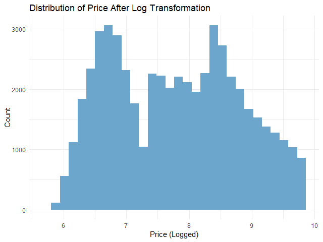
    # Check the distribution of logged `price`
    ggplot(dm,
           aes(x = price_log)) +
      
      ## Instantiate a histogram
      geom_histogram(fill = "skyblue3") +
      
      ## Add text elements
      labs(title = "Distribution of Price After Log Transformation",
           x = "Price (Logged)",
           y = "Count") +
      
      ## Set theme to minimal
      theme_minimal() 
    

    ผลลัพธ์:

    จะเห็นได้ว่า การกระจายตัวของตัวแปรตามใกล้เคียงกับการกระจายตัวแบบปกติมากขึ้นแล้ว

    .

    🚄 Step 3. Split the Data

    ในขั้นสุดท้ายก่อนใช้ linear regression เราจะแบ่งข้อมูลออกเป็น 2 ชุด:

    1. Training set สำหรับสร้าง linear regression model
    2. Test set สำหรับประเมินความสามารถของ linear regression model

    ในบทความนี้ เราจะแบ่ง 80% ของ dataset เป็น training set และ 20% เป็น test set:

    # Split the data
    
    ## Set seed for reproducibility
    set.seed(181)
    
    ## Training index
    train_index <- sample(nrow(dm),
                          0.8 * nrow(dm))
    
    ## Create training set
    train_set <- dm[train_index, ]
    
    ## Create test set
    test_set <- dm[-train_index, ]
    

    ตอนนี้ เราพร้อมที่จะสร้าง linear regression model กันแล้ว


    🏷️ Linear Regression Modelling

    การสร้าง linear regression model มีอยู่ 3 ขั้นตอน ได้แก่:

    1. Fit the model
    2. Make predictions
    3. Evaluate the model performance

    .

    💪 Step 1. Fit the Model

    ในขั้นแรก เราจะสร้าง model ด้วย lm() ซึ่งต้องการ input 2 อย่าง:

    lm(formula, data)
    1. formula = สูตรการทำนาย โดยเราต้องกำหนดตัวแปรต้นและตัวแปรตาม
    2. data = ชุดข้อมูลที่ใช้สร้าง model

    ในการทำนายราคาเพชร เราจะใช้ lm() แบบนี้:

    # Fit the model
    linear_reg <- lm(price_log ~ .,
                     data = train_set)
    

    อธิบาย code:

    • price_log ~ . หมายถึง ทำนายราคา (price_log) ด้วยตัวแปรต้นทั้งหมด (.)
    • data = train_set หมายถึง เรากำหนดชุดข้อมูลที่ใช้เป็น training set

    เราสามารถดูข้อมูลของ model ได้ด้วย summary():

    # View the model
    summary(linear_reg)
    

    ผลลัพธ์:

    Call:
    lm(formula = price_log ~ ., data = train_set)
    
    Residuals:
        Min      1Q  Median      3Q     Max 
    -2.2093 -0.0930  0.0019  0.0916  9.8935 
    
    Coefficients: (1 not defined because of singularities)
                     Estimate Std. Error  t value Pr(>|t|)    
    (Intercept)    -2.7959573  0.0705854  -39.611  < 2e-16 ***
    carat          -0.5270039  0.0086582  -60.867  < 2e-16 ***
    depth           0.0512357  0.0008077   63.437  < 2e-16 ***
    table           0.0090154  0.0005249   17.175  < 2e-16 ***
    x               1.1374016  0.0055578  204.651  < 2e-16 ***
    y               0.0290584  0.0031345    9.271  < 2e-16 ***
    z               0.0340298  0.0054896    6.199 5.73e-10 ***
    cutFair        -0.1528658  0.0060005  -25.476  < 2e-16 ***
    cutGood        -0.0639105  0.0036547  -17.487  < 2e-16 ***
    `cutVery Good` -0.0313800  0.0025724  -12.199  < 2e-16 ***
    cutPremium     -0.0451760  0.0026362  -17.137  < 2e-16 ***
    cutIdeal               NA         NA       NA       NA    
    colorE         -0.0573940  0.0032281  -17.779  < 2e-16 ***
    colorF         -0.0892633  0.0032654  -27.336  < 2e-16 ***
    colorG         -0.1573861  0.0032031  -49.136  < 2e-16 ***
    colorH         -0.2592763  0.0034037  -76.175  < 2e-16 ***
    colorI         -0.3864526  0.0038360 -100.742  < 2e-16 ***
    colorJ         -0.5258789  0.0047183 -111.455  < 2e-16 ***
    claritySI2      0.4431577  0.0079170   55.976  < 2e-16 ***
    claritySI1      0.6087513  0.0078819   77.234  < 2e-16 ***
    clarityVS2      0.7523161  0.0079211   94.976  < 2e-16 ***
    clarityVS1      0.8200656  0.0080463  101.918  < 2e-16 ***
    clarityVVS2     0.9381319  0.0082836  113.252  < 2e-16 ***
    clarityVVS1     1.0033931  0.0085098  117.910  < 2e-16 ***
    clarityIF       1.0898015  0.0092139  118.277  < 2e-16 ***
    ---
    Signif. codes:  0 ‘***’ 0.001 ‘**’ 0.01 ‘*’ 0.05 ‘.’ 0.1 ‘ ’ 1
    
    Residual standard error: 0.1825 on 43128 degrees of freedom
    Multiple R-squared:  0.9677,	Adjusted R-squared:  0.9676 
    F-statistic: 5.611e+04 on 23 and 43128 DF,  p-value: < 2.2e-16
    

    Note: ดูวิธีการอ่านผลลัพธ์ได้ที่ Explaining the lm() Summary in R และ Understanding Linear Regression Output in R

    .

    🔮 Step 2. Make Predictions

    ในขั้นที่สอง เราจะใช้ model เพื่อทำนายราคาด้วย predict():

    # Predict in the outcome space
    pred <- exp(pred_log)
    
    # Preview predictions
    head(pred_log)
    

    ผลลัพธ์:

           2        5        9       16       19       22 
    5.828071 5.816460 6.111859 5.777434 5.865820 6.088356
    

    จะเห็นว่า ราคาที่ทำนายยังอยู่ในรูป log ซึ่งเราต้องแปลงกลับเป็นราคาปกติด้วย exp():

    # Predict in the outcome space
    pred <- exp(pred_log)
    
    # Preview predictions
    head(pred)
    

    ผลลัพธ์:

           2        5        9       16       19       22 
    339.7028 335.7812 451.1766 322.9295 352.7713 440.6961 
    

    เราสามารถเปรียบเทียบราคาจริงกับราคาที่ทำนาย พร้อมความคลาดเคลื่อน ได้ดังนี้:

    # Compare predictions to actual
    results <- data.frame(actual = round(exp(test_set$price_log), 2),
                          predicted = round(pred, 2),
                          diff = round(exp(test_set$price_log) - pred, 2))
    
    # Print results
    head(results)
    

    ผลลัพธ์:

       actual predicted    diff
    2     326    339.70  -13.70
    5     335    335.78   -0.78
    9     337    451.18 -114.18
    16    345    322.93   22.07
    19    351    352.77   -1.77
    22    352    440.70  -88.70
    

    .

    🎯 Step 3. Evaluate the Model Performance

    ในขั้นสุดท้าย เราจะประเมิน model โดยใช้ 2 ตัวชี้วัด ได้แก่:

    1. Mean absolute error (MAE): ค่าเฉลี่ยความคลาดเคลื่อนโดยสัมบูรณ์
    2. Root mean squared error (RMSE): ค่าเฉลี่ยความคลาดเคลื่อนแบบยกกำลังสอง

    ทั้งสองตัวคำนวณความแตกต่างระหว่างสิ่งที่ทำนายและข้อมูลจริง ยิ่ง MAE และ RMSE สูง ก็หมายความว่า การทำนายมีความคาดเคลื่อนมาก แสดงว่า model ทำงานได้ไม่ดีนัก

    ในทางกลับกัน ถ้า MAE และ RMSE น้อย ก็แสดงว่า การทำนายใกล้เคียงกับข้อมูลจริง และ model มีความแม่นยำสูง

    (Note: เรียนรู้ความแตกต่างระหว่าง MAE และ RMSE ได้ที่ Loss Functions in Machine Learning Explained)

    เราสามารถคำนวณ MAE และ RMSE ได้ดังนี้:

    # Calculate MAE
    mae <- mean(abs(results$diff))
    
    # Calculate RMSE
    rmse <- sqrt(mean((results$diff)^2))
    
    # Print the results
    cat("MAE:", round(mae, 2), "\n")
    cat("RMSE:", round(rmse, 2))
    

    ผลลัพธ์:

    MAE: 491.71
    RMSE: 1123.68
    

    จากผลลัพธ์ เราจะเห็นว่า โดยเฉลี่ย model ทำนายราคาคลาดเคลื่อนไปประมาณ 492 ดอลล่าร์ (MAE)


    😎 Summary

    ในบทความนี้ เราได้ดูวิธีการทำ linear regression ในภาษา R กัน

    เราดูวิธีการเตรียมข้อมูลสำหรับ linear regression:

    1. One-hot encoding ด้วย model.matrix()
    2. Log transformation ด้วย log()
    3. Split data ด้วย sample()

    สร้าง linear regression model ด้วย lm() พร้อมประเมิน model ด้วย predict() และการคำนวณค่า MAE และ RMSE


    😺 GitHub

    ดู code ทั้งหมดในบทความนี้ได้ที่ GitHub


    📃 References


    ✅ R Book for Psychologists: หนังสือภาษา R สำหรับนักจิตวิทยา

    📕 ขอฝากหนังสือเล่มแรกในชีวิตด้วยนะครับ 😆

    🙋 ใครที่กำลังเรียนจิตวิทยาหรือทำงานสายจิตวิทยา และเบื่อที่ต้องใช้ software ราคาแพงอย่าง SPSS และ Excel เพื่อทำข้อมูล

    💪 ผมขอแนะนำ R Book for Psychologists หนังสือสอนใช้ภาษา R เพื่อการวิเคราะห์ข้อมูลทางจิตวิทยา ที่เขียนมาเพื่อนักจิตวิทยาที่ไม่เคยมีประสบการณ์เขียน code มาก่อน

    ในหนังสือ เราจะปูพื้นฐานภาษา R และพาไปดูวิธีวิเคราะห์สถิติที่ใช้บ่อยกัน เช่น:

    • Correlation
    • t-tests
    • ANOVA
    • Reliability
    • Factor analysis

    🚀 เมื่ออ่านและทำตามตัวอย่างใน R Book for Psychologists ทุกคนจะไม่ต้องพึง SPSS และ Excel ในการทำงานอีกต่อไป และสามารถวิเคราะห์ข้อมูลด้วยตัวเองได้ด้วยความมั่นใจ

    แล้วทุกคนจะแปลกใจว่า ทำไมภาษา R ง่ายขนาดนี้ 🙂‍↕️

    👉 สนใจดูรายละเอียดหนังสือได้ที่ meb:

  • วิธีวิเคราะห์และแปลผล principal component analysis (PCA) ในภาษา R — ตัวอย่างการใช้ prcomp() เพื่อลดตัวแปรใน wine dataset

    วิธีวิเคราะห์และแปลผล principal component analysis (PCA) ในภาษา R — ตัวอย่างการใช้ prcomp() เพื่อลดตัวแปรใน wine dataset

    ในบทความนี้ เราจะมาทำความรู้จักกับ principal component analysis (PCA) ในภาษา R กัน


    1. 🧐 PCA คืออะไร?
    2. 💻 PCA ในภาษา R
      1. 🧑‍💻 prcomp()
      2. 🍷 wine dataset
      3. ⚒️ PCA
      4. 📈 ดูผลลัพธ์
    3. 😺 GitHub
    4. 📃 References
    5. ✅ R Book for Psychologists: หนังสือภาษา R สำหรับนักจิตวิทยา

    🧐 PCA คืออะไร?

    PCA เป็น machine learning algorithm ประเภท unsupervised learning สำหรับลดตัวแปรในข้อมูล (dimensionality reduction) ในขณะที่ยังเก็บข้อมูลที่มีความสำคัญเอาไว้

    ยกตัวอย่างเช่น เรามีข้อมูลลูกค้าที่มี 50 ตัวแปร เช่น อายุ เงินเดือน ประวัติการใช้จ่าย ประวัติการเป็นสมาชิก … เราสามารถใช้ PCA เพื่อลดจำนวนตัวแปรลง เช่น ลดเหลือ 5 ตัวแปร ที่ยังให้ข้อมูลเกี่ยวกับลูกค้าได้เทียบเท่ากับ 50 ตัวแปร

    ในการทำงาน เราสามารถใช้ PCA เพื่อ:

    • ลดเวลาและ resource ในการประมวลผล เพราะมีตัวแปรที่ต้องประมวลผลน้อยลง
    • ช่วยทำความเข้าใจข้อมูล เพราะมีตัวแปรที่ต้องพิจารณาน้อยลง
    • ใช้เตรียมข้อมูลสำหรับสร้าง machine learning models อื่น ๆ เช่น regression model, hierarchical regression

    💻 PCA ในภาษา R

    .

    🧑‍💻 prcomp()

    ในภาษา R เราสามารถทำ PCA ได้ด้วย prcomp() ซึ่งเป็น function ใน base R (ซึ่งหมายความว่า เราไม่ต้องติดตั้ง package เพิ่มเติม)

    prcomp() ต้องการ 3 arguments ได้แก่:

    prcomp(x, center, scale.)
    • x คือ dataset ที่ต้องการใช้
    • center คือ ตัวเลือกว่า เราจะลบ mean ออกจากข้อมูลดิบ เพื่อให้ dataset มีค่า mean เป็น 0 ไหม (recommend ให้เป็น TRUE)
    • scale. คือ ตัวเลือกว่า เราจะหารข้อมูลดิบด้วย variance เพื่อให้ทุก column อยู่ในช่วงข้อมูลเดียวกันไหม (recommend ให้เป็น TRUE)

    .

    🍷 wine dataset

    เราลองมาดูตัวอย่าง PCA กับ wine dataset จาก rattle package กัน

    wine เป็นชุดข้อมูลที่มีลักษณะต่าง ๆ ของไวน์ เช่น ระดับแอลกอฮอล์ สี และความเข้มข้น

    (Note: ดูข้อมูลเพิ่มเติมเกี่ยวกับ wine dataset ได้ที่ wine: The wine dataset from the UCI Machine Learning Repository.)

    เราสามารถเรียกใช้ wine dataset ได้จาก rattle package ดังนี้:

    # Install and load the package
    
    ## Install
    install.packages("rattle")
    
    ## Load
    library(rattle)
    
    # -----------------------------------
    
    # Load the dataset
    
    ## Load
    data(wine)
    

    เรียกดูตัวอย่างข้อมูลใน wine dataset:

    # Preview
    head(wine)


    ผลลัพธ์:

      Type Alcohol Malic  Ash Alcalinity Magnesium Phenols Flavanoids Nonflavanoids Proanthocyanins Color  Hue Dilution Proline
    1    1   14.23  1.71 2.43       15.6       127    2.80       3.06          0.28            2.29  5.64 1.04     3.92    1065
    2    1   13.20  1.78 2.14       11.2       100    2.65       2.76          0.26            1.28  4.38 1.05     3.40    1050
    3    1   13.16  2.36 2.67       18.6       101    2.80       3.24          0.30            2.81  5.68 1.03     3.17    1185
    4    1   14.37  1.95 2.50       16.8       113    3.85       3.49          0.24            2.18  7.80 0.86     3.45    1480
    5    1   13.24  2.59 2.87       21.0       118    2.80       2.69          0.39            1.82  4.32 1.04     2.93     735
    6    1   14.20  1.76 2.45       15.2       112    3.27       3.39          0.34            1.97  6.75 1.05     2.85    1450
    

    ดูโครงสร้างของ wine dataset:

    # View the structure
    str(wine)
    

    ผลลัพธ์:

    'data.frame':	178 obs. of  14 variables:
     $ Type           : Factor w/ 3 levels "1","2","3": 1 1 1 1 1 1 1 1 1 1 ...
     $ Alcohol        : num  14.2 13.2 13.2 14.4 13.2 ...
     $ Malic          : num  1.71 1.78 2.36 1.95 2.59 1.76 1.87 2.15 1.64 1.35 ...
     $ Ash            : num  2.43 2.14 2.67 2.5 2.87 2.45 2.45 2.61 2.17 2.27 ...
     $ Alcalinity     : num  15.6 11.2 18.6 16.8 21 15.2 14.6 17.6 14 16 ...
     $ Magnesium      : int  127 100 101 113 118 112 96 121 97 98 ...
     $ Phenols        : num  2.8 2.65 2.8 3.85 2.8 3.27 2.5 2.6 2.8 2.98 ...
     $ Flavanoids     : num  3.06 2.76 3.24 3.49 2.69 3.39 2.52 2.51 2.98 3.15 ...
     $ Nonflavanoids  : num  0.28 0.26 0.3 0.24 0.39 0.34 0.3 0.31 0.29 0.22 ...
     $ Proanthocyanins: num  2.29 1.28 2.81 2.18 1.82 1.97 1.98 1.25 1.98 1.85 ...
     $ Color          : num  5.64 4.38 5.68 7.8 4.32 6.75 5.25 5.05 5.2 7.22 ...
     $ Hue            : num  1.04 1.05 1.03 0.86 1.04 1.05 1.02 1.06 1.08 1.01 ...
     $ Dilution       : num  3.92 3.4 3.17 3.45 2.93 2.85 3.58 3.58 2.85 3.55 ...
     $ Proline        : int  1065 1050 1185 1480 735 1450 1290 1295 1045 1045 ...
    

    Note: จะเห็นว่า ทุก column เป็นข้อมูลประเภท numeric ยกเว้น Type ที่ะเป็น factor

    .

    ⚒️ PCA

    หลังโหลด dataset แล้ว เราสามารถใช้ prcomp() เพื่อทำ PCA ได้ดังนี้:

    # PCA
    pca <- prcomp(wine[, -1],
                  center = TRUE,
                  scale. = TRUE)
    

    อธิบาย code:

    • เราใส่ wine[, -1] เพราะ PCA ใช้งานได้กับ column ที่เป็น numeric เท่านั้น เราเลย subset ข้อมูลเพื่อนำ Type ที่เป็น factor ออก
    • เรากำหนด center = TRUE เพื่อให้ mean เท่ากับ 0
    • กำหนดให้ scale. = TRUE เพื่อให้ข้อมูลอยู่ในช่วงข้อมูลเดียวกัน และป้องกันไม่ให้ข้อมูลที่อยู่ในมีช่วงข้อมูลกว้าง (เช่น ช่วง 1-100) มีผลต่อการวิเคราะห์มากกว่าข้อมูลที่มีช่วงแคบ (เช่น 1-10)

    .

    📈 ดูผลลัพธ์

    เราสามารถดูผลลัพธ์ของ PCA ได้ 2 วิธี ได้แก่:

    1. ดูค่าทางสถิติ
    2. สร้างกราฟ

    วิธีที่ 1. เราสามารถดูค่าทางสถิติได้ด้วย summary():

    # Print the results
    summary(pca)
    

    ผลลัพธ์:

    Importance of components:
                             PC1    PC2    PC3     PC4     PC5     PC6     PC7     PC8     PC9   PC10    PC11    PC12    PC13
    Standard deviation     2.169 1.5802 1.2025 0.95863 0.92370 0.80103 0.74231 0.59034 0.53748 0.5009 0.47517 0.41082 0.32152
    Proportion of Variance 0.362 0.1921 0.1112 0.07069 0.06563 0.04936 0.04239 0.02681 0.02222 0.0193 0.01737 0.01298 0.00795
    Cumulative Proportion  0.362 0.5541 0.6653 0.73599 0.80162 0.85098 0.89337 0.92018 0.94240 0.9617 0.97907 0.99205 1.00000
    

    ในผลลัพธ์ เราจะเห็นรายละเอียดดังนี้:

    • จำนวนตัวแปรที่ PCA สร้างให้ (PC ซึ่งย่อมาจาก principal component) ซึ่งในตัวอย่างมีทั้งหมด 13 ตัวแปร
    • Standard deviation (SD) ของแต่ละ PC
    • สัดส่วนข้อมูลที่อธิบายได้ด้วย PC แต่ละตัว (proportion of variance)
    • สัดส่วนข้อมูลสะสมที่อธิบายได้ เมื่อเพิ่ม PC แต่ละตัว (cumulative proportion) อย่างในตัวอย่าง จะเห็นว่า เมื่อเพิ่ม PC ตัวที่ 5 เราสามารถอธิบายข้อมูลได้ถึง 80% แล้ว แสดงว่า เราสามารถเก็บตัวแปรไว้ 5 จาก 13 ตัวแปรได้

    (Note: เราควรใช้ PC เท่ากับจำนวนที่สามารถอธิบายข้อมูลได้ตั้งแต่ 80% ขึ้นไป)

    วิธีที่ 2. เราสามารถดูผลลัพธ์ผ่านกราฟได้ เช่น scree plot ที่แสดงจำนวน PC และสัดส่วนข้อมูลสะสมที่อธิบายได้

    ในการเริ่มสร้างกราฟ ให้เราคำนวณหาสัดส่วน variance และสัดส่วนสะสมที่อธิบายได้ก่อน:

    # Extract variance explained
    pca_var <- pca$sdev^2
    pca_var_exp <- pca_var / sum(pca_var)
    
    # Compute cumulative variance explained
    cum_var_exp <- cumsum(pca_var_exp)
    

    จากนั้น นำผลลัพธ์ไปสร้างกราฟ:

    # Plot a scree plot for cumulative variance explained
    plot(cum_var_exp, 
         type = "b", col = "blue", pch = 19, lwd = 2,
         main = "Cumulative Variance Explained",
         xlab = "Number of Principal Components",
         ylab = "Cumulative Variance Explained",
         ylim = c(0, 1))
    

    ผลลัพธ์:

    จากกราฟ เราจะได้ข้อสรุปเดียวกันกับค่าทางสถิติ นั่นคือ เมื่อเรามี PC 5 ตัว เราจะสามารถอธิบายข้อมูลได้ถึง 80% ของข้อมูลเก่า


    😺 GitHub

    ดู code ทั้งหมดในบทความนี้ได้ที่ GitHub


    📃 References


    ✅ R Book for Psychologists: หนังสือภาษา R สำหรับนักจิตวิทยา

    📕 ขอฝากหนังสือเล่มแรกในชีวิตด้วยนะครับ 😆

    🙋 ใครที่กำลังเรียนจิตวิทยาหรือทำงานสายจิตวิทยา และเบื่อที่ต้องใช้ software ราคาแพงอย่าง SPSS และ Excel เพื่อทำข้อมูล

    💪 ผมขอแนะนำ R Book for Psychologists หนังสือสอนใช้ภาษา R เพื่อการวิเคราะห์ข้อมูลทางจิตวิทยา ที่เขียนมาเพื่อนักจิตวิทยาที่ไม่เคยมีประสบการณ์เขียน code มาก่อน

    ในหนังสือ เราจะปูพื้นฐานภาษา R และพาไปดูวิธีวิเคราะห์สถิติที่ใช้บ่อยกัน เช่น:

    • Correlation
    • t-tests
    • ANOVA
    • Reliability
    • Factor analysis

    🚀 เมื่ออ่านและทำตามตัวอย่างใน R Book for Psychologists ทุกคนจะไม่ต้องพึง SPSS และ Excel ในการทำงานอีกต่อไป และสามารถวิเคราะห์ข้อมูลด้วยตัวเองได้ด้วยความมั่นใจ

    แล้วทุกคนจะแปลกใจว่า ทำไมภาษา R ง่ายขนาดนี้ 🙂‍↕️

    👉 สนใจดูรายละเอียดหนังสือได้ที่ meb:

  • วิธีทำ Hierarchical Clustering ในภาษา R — ตัวอย่างการใช้ hclust() จัดกลุ่มข้อมูลอาชญากรรมจาก USArrests dataset

    วิธีทำ Hierarchical Clustering ในภาษา R — ตัวอย่างการใช้ hclust() จัดกลุ่มข้อมูลอาชญากรรมจาก USArrests dataset

    ในบทความนี้ เราจะมาทำความรู้จักกับ hierarchical cluster analysis (HCA) หรือ hierarchical clustering ในภาษา R กัน


    1. 🧐 HCA คืออะไร?
    2. 💻 HCA ในภาษา R: hclust()
    3. 🔢 Example Dataset: USArrests
    4. 📏 Normalise the Data
    5. 🍿 HCA With hclust()
    6. 📈 Print & Dendrogram
    7. 😺 GitHub
    8. 📃 References
    9. ✅ R Book for Psychologists: หนังสือภาษา R สำหรับนักจิตวิทยา

    🧐 HCA คืออะไร?

    HCA เป็น machine learning algorithm ประเภท unsupervised learning และใช้จัดกลุ่มข้อมูล (clustering) แบบลำดับชั้น (hierarchical)

    HCA มี 2 ประเภท:

    1. Agglomerative (bottom-up): จับ data point ที่อยู่ใกล้กันให้อยู่ cluster เดียวกัน แล้วจับ clusters ที่อยู่ใกล้กันให้อยูากลุ่มเดียวกัน ทำอย่างนี้ไปเรื่อย ๆ จนได้ 1 cluster ใหญ่
    2. Divisive (top-down): เริ่มจาก 1 cluster และแยก cluster ย่อยออกมาเรื่อย ๆ

    ตัวอย่างการใช้งาน HCA เช่น จัดกลุ่มผู้บริโภค (customer segmentation):


    💻 HCA ในภาษา R: hclust()

    ในภาษา R เราสามารถทำ HCA ได้ด้วย 2 functions:

    1. hclust() สำหรับ agglomerative HCA
    2. diana() จาก cluster package สำหรับ divisive HCA

    ในบทความนี้ เราจะดูวิธีใช้ hclust() ซึ่งเป็นที่นิยมสำหรับ HCA กัน


    🔢 Example Dataset: USArrests

    Dataset ที่เราจะใช้เป็นตัวอย่างในบทความนี้ คือ USArrests

    USArrests มีข้อมูลจำนวนประชากรจาก 50 รัฐในอเมริกา และข้อมูลการจับกุมใน 3 ประเภทการกระทำผิด ได้แก่:

    1. ฆาตกรรม (murder)
    2. ทำร้ายร่างกาย (assault)
    3. ข่มขืน (rape)

    ในการใช้งาน เราสามารถโหลด USArrests ได้ด้วย data():

    # Load
    data(USArrests)
    

    จากนั้น ดูตัวอย่างข้อมูลด้วย head():

    # Preview
    head(USArrests)
    

    ผลลัพธ์:

               Murder Assault UrbanPop Rape
    Alabama      13.2     236       58 21.2
    Alaska       10.0     263       48 44.5
    Arizona       8.1     294       80 31.0
    Arkansas      8.8     190       50 19.5
    California    9.0     276       91 40.6
    Colorado      7.9     204       78 38.7
    

    📏 Normalise the Data

    เนื่องจาก HCA จัดกลุ่มข้อมูลโดยใช้ระยะห่างระหว่างข้อมูล เราจะต้อง normalise ข้อมูล เพื่อให้ข้อมูลมีช่วงข้อมูลที่เท่า ๆ กัน และป้องกันไม่ให้ข้อมูลที่มีระยะห่างมาก (เช่น ข้อมูลที่อยู่ในช่วง 1 ถึง 1,000 เทียบกับ ข้อมูลที่มีช่วง 1 ถึง 10) มีผลต่อการจัดกลุ่ม

    สำหรับ HCA เราจะ normalise ด้วย z-score standardisation ซึ่งมีสูตรคำนวณดังนี้:

    Z = (X - M) / SD
    • Z = ข้อมูลที่ normalised แล้ว
    • X = ข้อมูลตั้งต้น
    • M = ค่าเฉลี่ยของข้อมูลตั้งต้น
    • SD = standard deviation (SD) ของข้อมูลตั้งต้น

    ทั้งนี้ เราสามารถทำ z-score standardisation ได้ด้วย scale():

    # Perform z-score standardisation
    USArrests_scaled <- scale(USArrests)
    

    จากนั้น เช็กผลลัพธ์ด้วย colMeans() และ apply() กับ sd():

    # Check the results
    
    ## Mean
    colMeans(USArrests_scaled)
    
    ## SD
    apply(USArrests_scaled, 2, sd)
    

    ผลลัพธ์:

    > ## Mean
    > round(colMeans(USArrests_scaled), 2)
      Murder  Assault UrbanPop     Rape 
           0        0        0        0 
    > 
    > ## SD
    > apply(USArrests_scaled, 2, sd)
      Murder  Assault UrbanPop     Rape 
           1        1        1        1 
    

    จะเห็นได้ว่า ทุก column มี mean เป็น 0 และ SD เป็น 1 แสดงว่า เรา normalise ข้อมูลได้สำเร็จ และพร้อมไปขั้นตอนถัดไป


    🍿 HCA With hclust()

    ตอนนี้ เราจะเริ่มใช้ HCA เพื่อจัดกลุ่มข้อมูลกัน

    hclust() ต้องการ input 2 อย่าง:

    hclust(d, method)

    Input #1. d หมายถึง distance matrix หรือ matrix ที่เก็บค่าระยะห่างระหว่างข้อมูลแบบ pair-wise ไว้

    เราสามารถคำนวณ distance matrix ได้ด้วย dist() function

    Input #2. method หมายถึง linkage method หรือวิธีในการจับ clusters รวมกันเป็น cluster ที่ใหญ่ขึ้น

    Linkage methods มี 5 ประเภท:

    1. Ward’s linkage: จับกลุ่ม cluster โดยลด variance ภายใน cluster
    2. Complete linkage: ใช้ระยะห่างสูงสุด
    3. Single linkage: ใช้ระยะห่างต่ำที่สุด
    4. Average linkage: ใช้ระยะห่างเฉลี่ยระหว่างข้อมูลจาก 2 clusters
    5. Centroid linkage: ใช้ระยะห่างระหว่างจุดศูนย์กลางของ 2 clusters

    Linkage ที่มักใช้กันได้ แก่ Ward’s, complete, และ average และในบทความนี้ เราจะใช้ Ward’s linkage ("ward.D2") กัน

    เราเรียกใช้ hclust() เพื่อจัดกลุ่มข้อมูล:

    # Create a distance matrix
    dm <- dist(USArrests_scaled)
    
    # HCA
    hc <- hclust(dm,
                 method = "ward.D2")
    

    ตอนนี้ เราก็ได้ข้อมูลที่จัดกลุ่มแล้ว


    สุดท้าย เราสามารถดูผลลัพธ์ของ HCA ได้ด้วย print():

    # Print HCA
    print(hc)
    

    ผลลัพธ์:

    Call:
    hclust(d = dm, method = "ward.D2")
    
    Cluster method   : ward.D2 
    Distance         : euclidean 
    Number of objects: 50 
    

    และการสร้าง dendrogram:

    # Plot a dendrogram
    plot(hc,
         hang = -1,
         cex = 0.8,
         main = "Dendrogram of USArrests Data")
    

    ผลลัพธ์:


    😺 GitHub

    ดู code ทั้งหมดในบทความนี้ได้ที่ GitHub


    📃 References


    ✅ R Book for Psychologists: หนังสือภาษา R สำหรับนักจิตวิทยา

    📕 ขอฝากหนังสือเล่มแรกในชีวิตด้วยนะครับ 😆

    🙋 ใครที่กำลังเรียนจิตวิทยาหรือทำงานสายจิตวิทยา และเบื่อที่ต้องใช้ software ราคาแพงอย่าง SPSS และ Excel เพื่อทำข้อมูล

    💪 ผมขอแนะนำ R Book for Psychologists หนังสือสอนใช้ภาษา R เพื่อการวิเคราะห์ข้อมูลทางจิตวิทยา ที่เขียนมาเพื่อนักจิตวิทยาที่ไม่เคยมีประสบการณ์เขียน code มาก่อน

    ในหนังสือ เราจะปูพื้นฐานภาษา R และพาไปดูวิธีวิเคราะห์สถิติที่ใช้บ่อยกัน เช่น:

    • Correlation
    • t-tests
    • ANOVA
    • Reliability
    • Factor analysis

    🚀 เมื่ออ่านและทำตามตัวอย่างใน R Book for Psychologists ทุกคนจะไม่ต้องพึง SPSS และ Excel ในการทำงานอีกต่อไป และสามารถวิเคราะห์ข้อมูลด้วยตัวเองได้ด้วยความมั่นใจ

    แล้วทุกคนจะแปลกใจว่า ทำไมภาษา R ง่ายขนาดนี้ 🙂‍↕️

    👉 สนใจดูรายละเอียดหนังสือได้ที่ meb:

  • วิธีจัดกลุ่มข้อมูลด้วย k-means ผ่าน kmeans() function ในภาษา R — ตัวอย่างการจัดกลุ่มหินจาก rock dataset

    วิธีจัดกลุ่มข้อมูลด้วย k-means ผ่าน kmeans() function ในภาษา R — ตัวอย่างการจัดกลุ่มหินจาก rock dataset

    ในบทความนี้ เราจะมาทำความรู้จักกับ k-means และวิธีใช้ kmeans() ในภาษา R กัน


    1. 👉 Introduction to k-Means
      1. 🤔 k-Means คืออะไร?
      2. 🪜 Steps การทำงานของ k-Means
      3. 🏫 Learn More
    2. 💻 k-Means ในภาษา R: kmeans()
    3. 🔢 Dataset
      1. 🪨 rock
      2. 📏 Data Normalisation
      3. 🔎 Finding the Optimal k
    4. ⏹️ k-Means
      1. 🔥 Train the Model
      2. 🤓 Get the Results
    5. 😺 GitHub
    6. 📃 References
    7. ✅ R Book for Psychologists: หนังสือภาษา R สำหรับนักจิตวิทยา

    👉 Introduction to k-Means

    .

    🤔 k-Means คืออะไร?

    k-means เป็น machine learning algorithm ประเภท unsupervised learning และใช้จัดกลุ่ม data (clustering) ที่เราไม่รู้จำนวนกลุ่มล่วงหน้า

    ตัวอย่างการใช้ k-means ในโลกจริง:

    • Customer segmentation: จัดกลุ่มลูกค้าที่เข้ามาซื้อสินค้า/บริการ
    • Anomaly detection: ตรวจจับความผิดปกติในคอมพิวเตอร์ (แบ่งกลุ่มกิจกรรมในคอมพิวเตอร์ เป็น “ปกติ” และ “ไม่ปกติ”)
    • Document clustering: จัดกลุ่มเอกสาร โดยอ้างอิงจากเนื้อหา

    .

    🪜 Steps การทำงานของ k-Means

    k-means มีการทำงานอยู่ 5 ขั้นตอน ได้แก่:

    1. กำหนดจำนวนกลุ่ม หรือ clusters (k)
    2. สุ่มวาง centroid หรือจุดศูนย์กลางของ cluster ลงในข้อมูล
    3. จัดกลุ่มข้อมูล โดยข้อมูลจะอยู่กลุ่มเดียวกับ centroid ที่ใกล้ที่สุด
    4. คำนวณหา centroid ใหม่
    5. ทำขั้นที่ 3 และ 4 ซ้ำ ตามจำนวนครั้งที่กำหนด หรือจนกว่าข้อมูลจะไม่เปลี่ยนกลุ่ม

    ตัวอย่างเช่น เราต้องการจัดกลุ่มข้อมูล 100 ตัวอย่าง:

    ขั้นที่ 1. เรากำหนด k เช่น ให้ k = 3

    ขั้นที่ 2. สุ่มวาง centroid (ดอกจันสีแดง) ลงในข้อมูล:

    ขั้นที่ 3. จัดข้อมูลให้อยู่กลุ่มเดียวกัน โดยอิงจาก centroid ที่อยู่ใกล้ที่สุด:

    ขั้นที่ 4. คำนวณหา centroids ใหม่:

    จะสังเกตเห็นว่า centroids ของเราเปลี่ยนไป

    ขั้นที่ 5. ทำขั้นที่ 3 และ 4 ซ้ำ ๆ ไปเรื่อย ๆ เช่น ทำไป 10 ครั้ง:

    เราก็จะได้การจัดกลุ่มข้อมูลมา

    .

    🏫 Learn More

    เรียนรู้เพิ่มเติมเกี่ยวกับ k-means ได้จากคอร์ส The Nuts and Bolts of Machine Learning จาก Google Career Certificates (เริ่มต้นที่ 1:33:49)


    💻 k-Means ในภาษา R: kmeans()

    ในภาษา R เราสามารถใช้ k-means ได้ผ่าน kmeans() function ซึ่งต้องการ 3 arguments หลัก ดังนี้:

    kmeans(x, centers, nstart)
    • x = dataset ที่ต้องการจัดกลุ่ม
    • centers = จำนวนกลุ่มข้อมูล หรือ k
    • nstart = จำนวนครั้งที่ k-means จะสุ่มวาง centroids ลงใน dataset เพื่อหาการจัดกลุ่มที่ดีที่สุด

    (Note: ศึกษา arguments เพิ่มเติมของ kmeans() ได้ที่ kmeans: K-Means Clustering)

    เราไปดูวิธีใช้งาน kmeans() กัน


    🔢 Dataset

    .

    🪨 rock

    ในบทความนี้ เราจะใช้ rock dataset ซึ่งเป็น built-in dataset ในภาษา R เป็นตัวอย่าง

    rock มีข้อมูลหิน 48 ตัวอย่าง และมีข้อมูลลักษณะ 4 อย่าง:

    ลำดับลักษณะคำอธิบาย
    1areaพื้นที่ผิว
    2periเส้นผ่านศูนย์กลาง
    3shapeขนาด (เส้นผ่านศูนย์กลาง หารด้วย พื้นที่ผิว)
    4permระดับความสามารถที่ให้น้ำซึมผ่านได้

    เป้าหมายของเรา คือ จัดกลุ่มหิน 48 ตัวอย่างตามลักษณะทั้งสี่

    เราสามารถโหลด rock dataset ได้โดยใช้ data() function:

    # Load
    data(rock)
    

    หลังจากโหลดแล้ว เราสามารถ preview ข้อมูลได้ด้วย head():

    # Preview the dataset
    head(rock)
    

    ผลลัพธ์:

      area    peri     shape perm
    1 4990 2791.90 0.0903296  6.3
    2 7002 3892.60 0.1486220  6.3
    3 7558 3930.66 0.1833120  6.3
    4 7352 3869.32 0.1170630  6.3
    5 7943 3948.54 0.1224170 17.1
    6 7979 4010.15 0.1670450 17.1
    

    .

    📏 Data Normalisation

    เนื่องจาก k-means ใช้ระยะห่างระหว่างข้อมูลในการจัดกลุ่ม ข้อมูลที่มีระยะห่างมาก (เช่น ระยะห่าง 500 เมตร กับ 1,000 เมตร) อาจมีผลต่อการจัดกลุ่มมากกว่าข้อมูลที่มีระยะห่างน้อย (เช่น ระยะห่าง 1 ซม. กับ 5 ซม.) และทำให้เกิด bias ในการจัดกลุ่มได้

    เพื่อป้องกัน bias เราควร normalise ข้อมูล หรือการปรับให้ข้อมูลอยู่ใน scale เดียวกัน

    สำหรับ k-means เรามักจะ normalise ข้อมูล ด้วย z-score standardisation ซึ่งมีสูตรการคำนวณดังนี้:

    Z = (X - M(X)) / SD(X)
    • Z = ข้อมูลที่ scaled แล้ว
    • X = ข้อมูลดิบ
    • M(X) = mean ของ X
    • SD(X) = SD ของ X

    ในภาษา R เราสามารถทำ z-score standardisation ได้ด้วย scale():

    # Scale
    rock_scaled <- scale(rock)
    

    Note: เราใส่ rock ไปใน argument และเก็บผลลัพธ์ไว้ใน data frame ใหม่ ชื่อ rock_scaled

    เราสามารถเช็กผลลัพธ์ได้ด้วย:

    • colMeans() เพื่อเช็ก mean
    • apply() และ sd() เพื่อเช็ก SD
    # Check the results
    
    ## Check mean
    round(colMeans(rock_scaled), 2)
    
    # Check SD
    apply(rock_scaled, 2, sd)
    

    ผลลัพธ์:

    > ### Check mean
    > round(colMeans(rock_scaled), 2)
     area  peri shape  perm 
        0     0     0     0 
    > 
    > ### Check SD
    > apply(rock_scaled, 2, sd)
     area  peri shape  perm 
        1     1     1     1 
    

    จากผลลัพธ์ เราจะเห็นได้ว่า ทุกลักษณะมี mean เท่ากับ 0 และ SD เท่ากับ 1 แสดงว่า เราทำ z-score standardisation ได้สำเร็จ และพร้อมไปขั้นตอนถัดไป

    .

    🔎 Finding the Optimal k

    ในการจัดกลุ่มด้วย k-means เราต้องเริ่มด้วยการกำหนด k

    แต่เราจะรู้ได้ยังไงว่า k ควรมีค่าเท่าไร?

    เรามี 3 วิธีในการหาค่า k ที่ดีที่สุด (optimal k):

    1. Elbow method
    2. Silhouette analysis
    3. Gap analysis

    ในบทความนี้ เราจะมาใช้วิธีแรกกัน: elbow method

    (Note: เรียนรู้เกี่ยวทั้งสามวิธีได้ที่ ML | Determine the optimal value of K in K-Means Clustering)

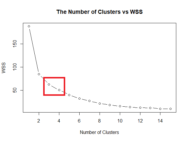
    Elbow method หาค่า k ที่ดีที่สุด โดยสร้างกราฟระหว่างค่า k และ within-cluster sum of squares (WSS) หรือระยะห่างระหว่างข้อมูลในกลุ่ม ค่า k ที่ดีที่สุด คือ ค่า k ที่ WSS เริ่มไม่ลดลง

    ในภาษา R เราสามารถเริ่มสร้างกราฟได้ โดยเริ่มจากใช้ for loop หา WSS สำหรับช่วงค่า k ที่เราต้องการ

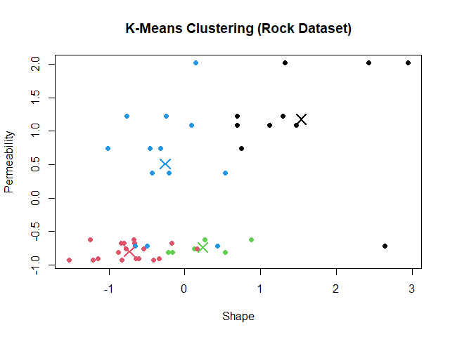
    ในตัวอย่าง rock dataset เราจะใช้ช่วงค่า k ระหว่าง 1 ถึง 15:

    # Initialise a vector for within cluster sum of squares (wss)
    wss <- numeric(15)
    
    # For-loop through the wss
    for (k in 1:15) {
      
      ## Try the k
      km <- kmeans(rock_scaled,
                   centers = k,
                   nstart = 20)
      
      ## Get WSS for the k
      wss[k] <- km$tot.withinss
    }
    

    จากนั้น ใช้ plot() สร้างกราฟความสัมพันธ์ระหว่างค่า k และ WSS:

    # Plot the wss
    plot(1:15,
         wss,
         type = "b",
         main = "The Number of Clusters vs WSS",
         xlab = "Number of Clusters",
         ylab = "WSS")
    

    ผลลัพธ์:

    จากกราฟ จะเห็นว่า WSS เริ่มชะลอตัว เมื่อค่า k อยู่ที่ 3 และ 4 ซึ่งเป็นจุดที่เป็นข้อศอก (elbow) ของกราฟ:

    แสดงว่า optimal k มีค่า 3 หรือ 4

    สำหรับบทความนี้ เราจะกำหนด optimal k = 4:

    # Set optiomal k = 4
    opt_k <- 4
    

    ⏹️ k-Means

    🔥 Train the Model

    หลังเตรียมข้อมูลและหา optimal k แล้ว เราก็พร้อมที่จะใช้ kmeans() ในการจัดกลุ่มข้อมูลแล้ว:

    # Set see for reproducibility
    set.seed(100)
    
    # Train the model
    km <- kmeans(rock_scaled,
                 centers = opt_k,
                 nstart = 20)
    

    .

    🤓 Get the Results

    เราสามารถดูผลการจัดกลุ่มได้ 2 วิธี:

    วิธีที่ 1. ดูค่าทางสถิติ:

    # Print the model
    print(km)
    

    ผลลัพธ์:

    K-means clustering with 4 clusters of sizes 10, 18, 6, 14
    
    Cluster means:
            area       peri
    1 -0.4406840 -0.9164442
    2  0.3496197  0.8022501
    3  1.5646450  1.3101981
    4 -0.8052989 -0.9383748
           shape       perm
    1  1.5369800  1.1775435
    2 -0.7319607 -0.8017914
    3  0.2358392 -0.7425075
    4 -0.2578245  0.5079897
    
    Clustering vector:
     [1] 2 2 2 2 2 2 2 2 2 2 2 2 3
    [14] 2 2 2 3 3 3 2 2 3 3 2 1 4
    [27] 4 4 4 1 1 1 4 1 4 1 4 1 4
    [40] 4 1 4 1 1 4 4 4 4
    
    Within cluster sum of squares by cluster:
    [1] 18.917267  8.104718
    [3]  1.471788 22.095636
     (between_SS / total_SS =  73.1 %)
    
    Available components:
    
    [1] "cluster"     
    [2] "centers"     
    [3] "totss"       
    [4] "withinss"    
    [5] "tot.withinss"
    [6] "betweenss"   
    [7] "size"        
    [8] "iter"        
    [9] "ifault"
    

    จากผลลัพธ์ จะเห็นได้ว่า ข้อมูลถูกแบ่งเป็น 4 กลุ่ม และเราสามารถดูค่า mean และ WSS ของแต่ละกลุ่มได้

    .

    วิธีที่ 2. สร้างกราฟ:

    # Create a plot
    plot(rock_scaled[, c("shape", "perm")], 
         col = km$cluster,
         pch = 19,
         main = "K-Means Clustering (Rock Dataset)",
         xlab = "Shape",
         ylab = "Permeability")
    
    # Add cluster centers
    points(km$centers[, c("shape", "perm")], 
           col = 1:5,
           pch = 4,
           cex = 2,
           lwd = 2)
    

    ผลลัพธ์:

    ตอนนี้ เราก็ได้ข้อมูลที่จัดกลุ่มด้วย k-means เรียบร้อยแล้ว 👍


    😺 GitHub

    ดู code ทั้งหมดในบทความนี้ได้ที่ GitHub


    📃 References


    ✅ R Book for Psychologists: หนังสือภาษา R สำหรับนักจิตวิทยา

    📕 ขอฝากหนังสือเล่มแรกในชีวิตด้วยนะครับ 😆

    🙋 ใครที่กำลังเรียนจิตวิทยาหรือทำงานสายจิตวิทยา และเบื่อที่ต้องใช้ software ราคาแพงอย่าง SPSS และ Excel เพื่อทำข้อมูล

    💪 ผมขอแนะนำ R Book for Psychologists หนังสือสอนใช้ภาษา R เพื่อการวิเคราะห์ข้อมูลทางจิตวิทยา ที่เขียนมาเพื่อนักจิตวิทยาที่ไม่เคยมีประสบการณ์เขียน code มาก่อน

    ในหนังสือ เราจะปูพื้นฐานภาษา R และพาไปดูวิธีวิเคราะห์สถิติที่ใช้บ่อยกัน เช่น:

    • Correlation
    • t-tests
    • ANOVA
    • Reliability
    • Factor analysis

    🚀 เมื่ออ่านและทำตามตัวอย่างใน R Book for Psychologists ทุกคนจะไม่ต้องพึง SPSS และ Excel ในการทำงานอีกต่อไป และสามารถวิเคราะห์ข้อมูลด้วยตัวเองได้ด้วยความมั่นใจ

    แล้วทุกคนจะแปลกใจว่า ทำไมภาษา R ง่ายขนาดนี้ 🙂‍↕️

    👉 สนใจดูรายละเอียดหนังสือได้ที่ meb:

  • สอนปลูกต้นไม้ในภาษา R (ภาค 1): วิธีสร้าง tree-based models ใน 3 ขั้นตอนด้วย rpart และ randomForest packages — ตัวอย่างการทำนายประเภทเกียร์รถใน mtcars dataset

    สอนปลูกต้นไม้ในภาษา R (ภาค 1): วิธีสร้าง tree-based models ใน 3 ขั้นตอนด้วย rpart และ randomForest packages — ตัวอย่างการทำนายประเภทเกียร์รถใน mtcars dataset

    ในบทความนี้ เราจะมาทำความรู้จักและสร้าง tree-based models ในภาษา R กัน:

    1. Classification tree
    2. Random forest

    ถ้าพร้อมแล้ว ไปเริ่มกันเลย


    🌳 Tree-Based Algorithms คืออะไร?

    Tree-based algorithm เป็น machine learning algorithm ประเภท supervised learning ที่ทำนายข้อมูลโดยใช้ decision tree

    Decision tree เป็นเครื่องมือช่วยตัดสินใจที่ดูคล้ายกับต้นไม้กลับหัว เพราะประกอบด้วยจุดตัดสินใจ (node) ที่แตกยอด (ทางเลือก) ออกไปเรื่อย ๆ เพื่อใช้ทำนายผลลัพธ์ที่ต้องการ

    ยกตัวอย่างเช่น เราอยากรู้ว่า เราควรจะสมัครงานกับบริษัทแห่งหนึ่งไหม เราอาจจะสร้าง decision tree จาก 3 ปัจจัย คือ:

    1. เงินเดือน
    2. ได้ใช้ทักษะที่มี
    3. การทำงานแบบ hybrid หรือ remote

    ได้แบบนี้:

    จาก decision tree ถ้าเราเห็นงานที่ได้เงินเดือนไม่ตรงใจ เราจะไม่สมัครงานนั้น (เส้นการตัดสินใจซ้ายสุด)

    ในทางกลับกัน ถ้างานมีเงินเดือนที่น่าสนใจ และได้ใช้ทักษะที่มีอยู่ เราจะสมัครงานนั้น (เส้นการตัดสินใจขวาสุด) เป็นต้น


    💻 Tree-Based Models ในภาษา R

    ในภาษา R เราสามารถสร้าง tree-based model ได้ด้วย rpart() จาก rpart package:

    # Install
    install.packages("rpart")
    # Load
    library(rpart)
    

    rpart() ต้องการ 4 arguments ดังนี้:

    rpart(formula, data, method, control)
    • formula = สูตรในการวิเคราะห์ (ตัวแปรตาม ~ ตัวแปรต้น)
    • data = dataset ที่ใช้สร้าง model
    • method = ประเภท algorithm ("anova" สำหรับ regression และ "class" สำหรับ classification)
    • control (optional) = เงื่อนไขควบคุม “การเติบโต” ของ decision tree เช่น ระดับชั้นที่มีได้ เป็นต้น

    (Note: ศึกษาการใช้งาน rpart() เพิ่มเติมได้ที่ rpart: Recursive Partitioning and Regression Trees)

    เราไปดูตัวอย่างการใช้งาน rpart() กัน

    .

    🚗 Dataset: mtcars

    ในบทความนี้ เราจะลองสร้าง tree-based model ประเภท classification หรือ classification tree เพื่อทำนายประเภทเกียร์รถใน mtcars dataset

    mtcars เป็นชุดข้อมูลรถจาก ปี ค.ศ. 1974 ซึ่งประกอบไปด้วยข้อมูล เช่น รุ่นรถ น้ำหนัก ระดับการกินน้ำมัน แรงม้า เป็นต้น

    เราสามารถโหลด mtcars มาใช้งานได้ด้วย data() และ preview ด้วย head():

    # Load
    data(mtcars)
    # Preview
    head(mtcars)
    

    ตัวอย่างข้อมูล:

                       mpg cyl disp  hp drat    wt  qsec vs        am gear carb
    Mazda RX4         21.0   6  160 110 3.90 2.620 16.46  0    manual    4    4
    Mazda RX4 Wag     21.0   6  160 110 3.90 2.875 17.02  0    manual    4    4
    Datsun 710        22.8   4  108  93 3.85 2.320 18.61  1    manual    4    1
    Hornet 4 Drive    21.4   6  258 110 3.08 3.215 19.44  1 automatic    3    1
    Hornet Sportabout 18.7   8  360 175 3.15 3.440 17.02  0 automatic    3    2
    Valiant           18.1   6  225 105 2.76 3.460 20.22  1 automatic    3    1
    

    .

    🔧 Prepare the Data

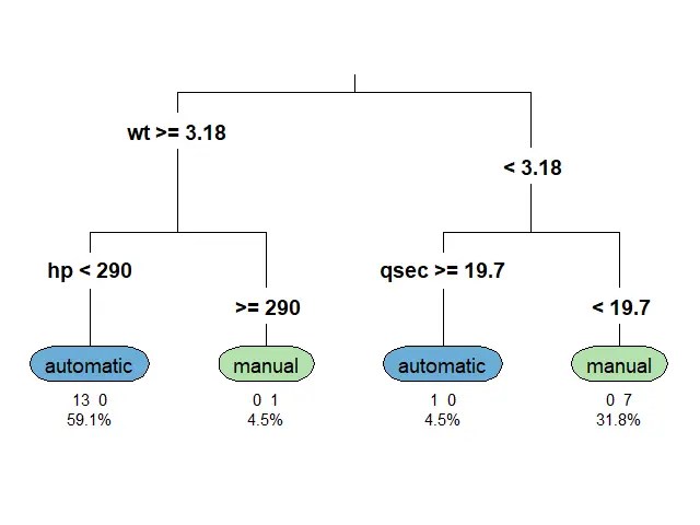
    ก่อนนำ mtcars ไปใช้สร้าง classification tree เราจะต้องทำ 2 อย่างก่อน:

    อย่างที่ #1. ปรับ column am ให้เป็น factor เพราะสิ่งที่เราต้องการทำนายเป็น categorical data:

    # Convert `am` to factor
    mtcars$am <- factor(mtcars$am,
                        levels = c(0, 1),
                        labels = c("automatic", "manual"))
    # Check the result
    class(mtcars$am)
    

    ผลลัพธ์:

    [1] "factor"
    

    อย่างที่ #2. Split ข้อมูลเป็น 2 ชุด:

    1. Training set สำหรับสร้าง model
    2. Test set สำหรับประเมิน model
    # Set seed for reproducibility
    set.seed(500)
    # Get training index
    train_index <- sample(nrow(mtcars),
                          nrow(mtcars) * 0.7)
    # Split the data
    train_set <- mtcars[train_index, ]
    test_set <- mtcars[-train_index, ]
    

    .

    🪴 Train the Model

    ตอนนี้ เราพร้อมที่จะสร้าง classification tree ด้วย rpart() แล้ว

    สำหรับ classification tree ในบทความนี้ เราจะลองตั้งเงื่อนไขในการปลูกต้นไม้ (control) ดังนี้:

    ArgumentExplanation
    cp = 0คะแนนประสิทธิภาพขั้นต่ำ ก่อนจะแตกกิ่งใหม่ได้ = 0
    minsplit = 1จำนวนกิ่งย่อยขั้นต่ำที่ต้องมี ก่อนจะแตกกิ่งใหม่ได้ = 1
    maxdepth = 5จำนวนชั้นที่ decision tree มีได้สูงสุด = 5
    # Classification tree
    ct <- rpart(am ~ .,
                data = train_set,
                method = "class",
                control = rpart.control(cp = 0, minsplit = 1, maxdepth = 5))
    

    เราสามารถดู classification tree ของเราได้ด้วย rpart.plot():

    # Plot classification tree
    rpart.plot(ct,
               type = 3,
               extra = 101,
               under = TRUE,
               digits = 3,
               tweak = 1.2)
    

    ผลลัพธ์:

    Note:

    • ก่อนใช้งาน rpart.plot() เราต้องจะติดตั้งและเรียกใช้งานด้วย install.packages() และ library() ตามลำดับ
    • ศึกษาการใช้งาน rpart.plot() เพิ่มเติมได้ที่ rpart.plot: Plot an rpart model. A simplified interface to the prp function.

    .

    📏 Evaluate the Model

    เมื่อได้ classification tree มาแล้ว เราลองมาประเมินความสามารถของ model ด้วย accuracy หรือสัดส่วนการทำนายที่ถูกต้องกัน

    เราเริ่มจากใช้ predict() เพื่อใช้ model ทำนายประเภทเกียร์:

    # Predict the outcome
    test_set$pred_ct <- predict(ct,
                                newdata = test_set,
                                type = "class")
    

    จากนั้น สร้าง confusion matrix หรือ matrix เปรียบเทียบคำทำนายกับข้อมูลจริง:

    # Create a confusion matrix
    cm_ct <- table(Predicted = test_set$pred_ct,
                   Actual = test_set$am)
    # Print confusion matrix
    print(cm_ct)
    

    ผลลัพธ์:

               Actual
    Predicted   automatic manual
      automatic         5      1
      manual            0      4
    

    สุดท้าย เราหา accuracy ด้วยการนำจำนวนคำทำนายที่ถูกต้องมาหารด้วยจำนวนคำทำนายทั้งหมด:

    # Get accuracy
    acc_ct <- sum(diag(cm_ct)) / sum(cm_ct)
    # Print accuracy
    cat("Accuracy (classification tree):", acc_ct)
    

    ผลลัพธ์:

    Accuracy (classification tree): 0.9
    

    จะเห็นได้ว่า model ของเรามีความแม่นยำถึง 90%


    🍄 Random Forest

    Random forest เป็น tree-based algorithm ที่ช่วยเพิ่มความแม่นยำในการทำนาย โดยสุ่มสร้าง decision trees ต้นเล็กขึ้นมาเป็นกลุ่ม (forest) แทนการปลูก decision tree ต้นเดียว

    Decision tree แต่ละต้นใน random forest มีความสามารถในการทำนายแตกต่างกัน ซึ่งบางต้นอาจมีความสามารถที่น้อยมาก

    แต่จุดแข็งของ random forest อยู่ที่จำนวน โดย random forest ทำนายผลลัพธ์โดยดูจากผลลัพธ์ในภาพรวม ดังนี้:

    TaskPredict by
    Regressionค่าเฉลี่ยของผลลัพธ์การทำนายของทุกต้น
    Classificationเสียงส่วนมาก (majority vote)

    ดังนั้น แม้ว่า decision tree บางต้นอาจทำนายผิดพลาด แต่โดยรวมแล้ว random forest มีโอกาสที่จะทำนายได้ดีกว่า decision tree ต้นเดียว

    ในภาษา R เราสามารถสร้าง random forest ได้ด้วย randomForest() จาก randomForest package ซึ่งต้องการ 3 arguments:

    randomFrest(formula, data, ntree)
    • formula = สูตรในการวิเคราะห์ (ตัวแปรตาม ~ ตัวแปรต้น)
    • data = dataset ที่ใช้สร้าง model
    • ntree = จำนวน decision trees ที่ต้องการสร้าง

    Note:

    • เราไม่ต้องกำหนดว่า จะทำ classification หรือ regression model เพราะ randomForest() จะเลือก model ให้อัตโนมัติตามข้อมูลที่เราใส่เข้าไป
    • ศึกษาการใช้งาน randomForest() เพิ่มเติมได้ที่ randomForest: Classification and Regression with Random Forest

    ก่อนใช้ randomForest() เราต้องเตรียมข้อมูลแบบเดียวกันกับ rpart() ได้แก่:

    1. เปลี่ยน am ให้เป็น factor
    2. Split the data

    สมมุติว่า เราเตรียมข้อมูลแล้ว เราสามารถเรียกใช้ randomForest() ได้เลย โดยเราจะลองสร้าง random forest ที่ประกอบด้วย decision trees 100 ต้น:

    # Random forest
    rf <- randomForest(am ~ .,
                       data = train_set,
                       ntree = 100)
    

    แล้วลองประเมินความสามารถของ model ด้วย accuracy

    เริ่มจากทำนายประเภทเกียร์:

    # Predict the outcome
    test_set$pred_rf <- predict(rf,
                                newdata = test_set,
                                type = "class")
    

    สร้าง confusion matrix:

    # Create a confusion matrix
    cm_rf <- table(Predicted = test_set$pred_rf,
                   Actual = test_set$am)
    # Print confusion matrix
    print(cm_rf)
    

    ผลลัพธ์:

               Actual
    Predicted   automatic manual
      automatic         5      0
      manual            0      5
    

    และสุดท้าย คำนวณ accuracy:

    # Get accuracy
    acc_rf <- sum(diag(cm_rf)) / sum(cm_rf)
    # Print accuracy
    cat("Accuracy (random forest):", acc_rf)
    

    ผลลัพธ์:

    Accuracy (random forest): 1
    

    จะเห็นว่า random forest (100%) มีความแม่นยำในการทำนายมากกว่า classification tree ต้นเดียว (90%)


    🐱 GitHub

    ดู code ทั้งหมดในบทความนี้ได้ที่ GitHub:


    📃 References


    ✅ R Book for Psychologists: หนังสือภาษา R สำหรับนักจิตวิทยา

    📕 ขอฝากหนังสือเล่มแรกในชีวิตด้วยนะครับ 😆

    🙋 ใครที่กำลังเรียนจิตวิทยาหรือทำงานสายจิตวิทยา และเบื่อที่ต้องใช้ software ราคาแพงอย่าง SPSS และ Excel เพื่อทำข้อมูล

    💪 ผมขอแนะนำ R Book for Psychologists หนังสือสอนใช้ภาษา R เพื่อการวิเคราะห์ข้อมูลทางจิตวิทยา ที่เขียนมาเพื่อนักจิตวิทยาที่ไม่เคยมีประสบการณ์เขียน code มาก่อน

    ในหนังสือ เราจะปูพื้นฐานภาษา R และพาไปดูวิธีวิเคราะห์สถิติที่ใช้บ่อยกัน เช่น:

    • Correlation
    • t-tests
    • ANOVA
    • Reliability
    • Factor analysis

    🚀 เมื่ออ่านและทำตามตัวอย่างใน R Book for Psychologists ทุกคนจะไม่ต้องพึง SPSS และ Excel ในการทำงานอีกต่อไป และสามารถวิเคราะห์ข้อมูลด้วยตัวเองได้ด้วยความมั่นใจ

    แล้วทุกคนจะแปลกใจว่า ทำไมภาษา R ง่ายขนาดนี้ 🙂‍↕️

    👉 สนใจดูรายละเอียดหนังสือได้ที่ meb:

  • วิธีสร้าง Naïve Bayes classifier ใน 5 ขั้นตอนด้วย naivebayes package ในภาษา R – ตัวอย่างการทำนายประเภทดอกไม้ใน iris dataset

    วิธีสร้าง Naïve Bayes classifier ใน 5 ขั้นตอนด้วย naivebayes package ในภาษา R – ตัวอย่างการทำนายประเภทดอกไม้ใน iris dataset

    ในบทความนี้ เราจะมาทำความรู้กับ Naïve Bayes และดูวิธีสร้าง Naïve Bayes classifier ในภาษา R ด้วย naivebayes package กัน


    1. 👼 Naïve Bayes คืออะไร?
    2. 🧑‍💻 วิธีสร้าง NB Classifer ด้วย naivebayes Package
      1. 1️⃣ Step 1. Install & Load the Package
      2. 2️⃣ Step 2. Load & Preview the Dataset
      3. 3️⃣ Step 3. Split the Dataset
      4. 4️⃣ Step 4. Create a NB Model
      5. 5️⃣ Step 5. Evaluate the Model
    3. 😺 GitHub
    4. 📃 References
    5. ✅ R Book for Psychologists: หนังสือภาษา R สำหรับนักจิตวิทยา

    👼 Naïve Bayes คืออะไร?

    Naïve Bayes (NB) เป็น machine learning algorithm ประเภท supervised learning สำหรับทำนายกลุ่มของข้อมูล (classification)

    NB ทำนายข้อมูล โดยวิเคราะห์ความน่าจะเป็นที่ 2 เหตุการณ์ (ตัวแปรต้นและตัวแปรตาม) จะเกิดขึ้นคู่กัน

    ยกตัวอย่างเช่น การอนุมัติสินเชื่อ (อนุมัติ/ไม่อนุมัติ) ที่เกิดขึ้นอยู่กับ:

    • รายได้: รายได้มาก -> อนุมัติ
    • อายุ: อายุน้อย -> อนุมัติ
    • ประวัติการขอสินเชื่อ: เคยขอแล้วผ่าน -> อนุมัติ

    NB คำนวณความน่าจะเป็นของแต่ละปัจจัยต่อตัวแปรตาม (การอนุมัติ) โดยอนุมานว่า แต่ละปัจจัยเกิดแยกกัน (independent) แม้ว่าในความเป็นจริงหลายปัจจัยจะเกิดขึ้นร่วมกัน (dependent; เช่น อายุมาก -> รายได้มาก) ก็ตาม

    เนื่องจาก NB มีการมองโลกอย่างง่าย จึงได้ชื่อว่า “naïve” หรือไร้เดียงนั่นเอง

    แม้ว่า NB จะมีการมองโลกที่ไร้เดียงสา แต่ก็เป็น algorithm ที่:

    1. เข้าใจได้ง่าย (เพราะไร้เดียงสา)
    2. รวดเร็ว (เพราะใช้การวิเคราะห์อย่างง่าย)
    3. น่าเชื่อถือ (มักจะทำนายได้แม่นยำ แม้จะมีมุมมองที่ไม่ตรงกับความเป็นจริง)

    🧑‍💻 วิธีสร้าง NB Classifer ด้วย naivebayes Package

    วิธีการสร้าง NB classifier ด้วย naivebayes package มี 5 ขั้นตอน ได้แก่:

    1. Install and load the package
    2. Load and preview the dataset
    3. Split the dataset
    4. Create a NB model
    5. Evaluate the model

    .

    1️⃣ Step 1. Install & Load the Package

    ในขั้นแรก เราต้องติดตั้งและเรียกใช้งาน naivebayes package:

    # Install and load the package
    ## Install
    install.packages("naivebayes")
    ## Load
    library(naivebayes)
    

    Note: เราทำการติดตั้งแค่ครั้งแรกครั้งเดียว แต่การเรียกใช้ต้องทำทุกครั้งทุกเริ่ม session ใหม่

    .

    2️⃣ Step 2. Load & Preview the Dataset

    ในขั้นที่สอง ให้เราโหลด dataset ที่จะใช้งาน

    โดยในบทความนี้ เราจะใช้ built-in dataset ในภาษา R ชื่อ iris dataset

    iris dataset มีกลีบดอกของข้อมูลดอกไม้ 3 ชนิด ได้แก่:

    • Iris setosa
    • Iris virginica
    • Iris versicolor

    เป้าหมายของเรา คือ ทำนายประเภทของดอกไม้จากความกว้างและความยาวกลีบดอก

    เนื่องจากเป็น built-in dataset เราสามารถโหลด iris dataset ด้วยคำสั่ง data():

    # Load
    data(iris)
    

    จากนั้น เราสามารถใช้คำสั่ง head() เพื่อ preview ข้อมูล:

    # Preview
    head(iris)
    

    ผลลัพธ์:

      Sepal.Length Sepal.Width Petal.Length Petal.Width Species
    1          5.1         3.5          1.4         0.2  setosa
    2          4.9         3.0          1.4         0.2  setosa
    3          4.7         3.2          1.3         0.2  setosa
    4          4.6         3.1          1.5         0.2  setosa
    5          5.0         3.6          1.4         0.2  setosa
    6          5.4         3.9          1.7         0.4  setosa
    

    Note: จะเห็นว่า iris dataset มีข้อมูลทั้งหมด 5 columns คือ ความยาวและความกว้างของกลีบดอกชั้นนอก (sepal) และความยาวและความกว้างของกลีบดอกชั้นใน (petal) รวมทั้งประเภทดอกไม้ (species)

    เนื่องจาก NB classifier ต้องการตัวแปรตามที่เป็น factor เราต้องเช็กได้ว่า Species เป็น data type ไหนด้วยคำสั่ง str():

    # Preview
    str(iris)
    

    ผลลัพธ์:

    'data.frame':	150 obs. of  5 variables:
     $ Sepal.Length: num  5.1 4.9 4.7 4.6 5 5.4 4.6 5 4.4 4.9 ...
     $ Sepal.Width : num  3.5 3 3.2 3.1 3.6 3.9 3.4 3.4 2.9 3.1 ...
     $ Petal.Length: num  1.4 1.4 1.3 1.5 1.4 1.7 1.4 1.5 1.4 1.5 ...
     $ Petal.Width : num  0.2 0.2 0.2 0.2 0.2 0.4 0.3 0.2 0.2 0.1 ...
     $ Species     : Factor w/ 3 levels "setosa","versicolor",..: 1 1 1 1 1 1 1 1 1 1 ...
    

    จะเห็นได้ว่า Species เป็น factor อยู่แล้ว และพร้อมที่ใช้สร้าง NB classifier

    .

    3️⃣ Step 3. Split the Dataset

    ในขั้นที่สาม เราจะแบ่งข้อมูลเป็น 2 ชุด:

    1. Training set เพื่อสร้าง NB classifier
    2. Test set เพื่อทดสอบประสิทธิภาพของ NB classifier

    ขั้นแรกในการแบ่งข้อมูล ให้เราสุ่มเลือก row index ที่จะอยู่ใน training set:

    # Set seed for reproducibility
    set.seed(2025)
    # Create a training index
    training_index <- sample(1:nrow(iris),
                             0.7 * nrow(iris))
    

    จากนั้น ใช้ row index ที่ได้แบ่งข้อมูลเป็น 2 ชุด:

    # Split the dataset
    train_set <- iris[training_index, ]
    test_set <- iris[-training_index, ]
    

    .

    4️⃣ Step 4. Create a NB Model

    ในขั้นที่สี่ เราจะสร้าง NB classifier โดยใช้ naive_bayes() จาก naivebayes package

    naive_bayes() ต้องการ input 2 อย่าง:

    1. Formula: ตัวแปรต้นและตัวแปรตามที่ต้องการใช้สร้าง model โดยในกรณีนี้ คือ ทำนาย Species ด้วยข้อมูลที่เหลือทั้งหมด (.)
    2. Data: dataset ที่จะใช้สร้าง model ซึ่งในกรณีนี้ คือ train_set
    # Create a NB model
    nb <- naive_bayes(Species ~ .,
                      data = train_set)
    

    เมื่อเราได้ NB classifier มาแล้ว เรามาลองใช้ model ทำนายประเภทดอกไม้กัน:

    # Predict the outcomes
    pred <- predict(nb,
                    newdata = test_set[, 1:4],
                    type = "class")
    print(pred)
    

    ผลลัพธ์:

     [1] setosa     setosa     setosa     setosa     setosa    
     [6] setosa     setosa     setosa     setosa     setosa    
    [11] setosa     setosa     setosa     setosa     setosa    
    [16] virginica  versicolor versicolor versicolor versicolor
    [21] virginica  versicolor versicolor versicolor versicolor
    [26] versicolor virginica  versicolor versicolor versicolor
    [31] versicolor versicolor versicolor versicolor virginica 
    [36] virginica  virginica  virginica  virginica  virginica 
    [41] virginica  virginica  virginica  virginica  virginica 
    Levels: setosa versicolor virginica
    

    .

    5️⃣ Step 5. Evaluate the Model

    ในขั้นสุดท้าย เราจะประเมินประสิทธิภาพของ model ด้วยการคำนวณ accuracy หรือ สัดส่วนของคำตอบที่ model ตอบถูก:

    Accuracy = Correct predictions / Total predictions

    เราสามารถหาค่า accuracy ได้โดยเริ่มสร้าง confusion matrix ก่อน:

    # Create a confusion matrix
    cm <- table(Predicted = pred, 
                Actual = test_set$Species)
    print(cm)
    

    ผลลัพธ์:

                Actual
    Predicted    setosa versicolor virginica
      setosa         15          0         0
      versicolor      0         16         0
      virginica       0          3        11
    

    จากนั้น นำจำนวนคำตอบที่ถูกต้องและจำนวนคำตอบทั้งหมดมาหาค่า accuracy:

    # Calculate the accuracy
    accuracy <- sum(diag(cm)) / sum(cm)
    cat("Accuracy:", round(accuracy, 2))
    

    ผลลัพธ์:

    Accuracy: 0.93
    

    จะเห็นได้ว่า NB classifier ที่เป็น model ไร้เดียงสาของเรา มีความแม่นยำในการทำนายสูงถึง 93%


    😺 GitHub

    ดู code ทั้งหมดในบทความนี้ได้ที่ GitHub


    📃 References


    ✅ R Book for Psychologists: หนังสือภาษา R สำหรับนักจิตวิทยา

    📕 ขอฝากหนังสือเล่มแรกในชีวิตด้วยนะครับ 😆

    🙋 ใครที่กำลังเรียนจิตวิทยาหรือทำงานสายจิตวิทยา และเบื่อที่ต้องใช้ software ราคาแพงอย่าง SPSS และ Excel เพื่อทำข้อมูล

    💪 ผมขอแนะนำ R Book for Psychologists หนังสือสอนใช้ภาษา R เพื่อการวิเคราะห์ข้อมูลทางจิตวิทยา ที่เขียนมาเพื่อนักจิตวิทยาที่ไม่เคยมีประสบการณ์เขียน code มาก่อน

    ในหนังสือ เราจะปูพื้นฐานภาษา R และพาไปดูวิธีวิเคราะห์สถิติที่ใช้บ่อยกัน เช่น:

    • Correlation
    • t-tests
    • ANOVA
    • Reliability
    • Factor analysis

    🚀 เมื่ออ่านและทำตามตัวอย่างใน R Book for Psychologists ทุกคนจะไม่ต้องพึง SPSS และ Excel ในการทำงานอีกต่อไป และสามารถวิเคราะห์ข้อมูลด้วยตัวเองได้ด้วยความมั่นใจ

    แล้วทุกคนจะแปลกใจว่า ทำไมภาษา R ง่ายขนาดนี้ 🙂‍↕️

    👉 สนใจดูรายละเอียดหนังสือได้ที่ meb: