Tag: Hyperparametre tuning

tidymodels: แนะนำวิธีใช้แพ็กเกจ machine learning ที่ทรงพลัง ครบจบ และทันสมัยในภาษา R เพื่อสร้าง ประเมิน และปรับทูน model — ตัวอย่างการทำนายราคาบ้านใน Boston dataset

ในการทำ machine learning (ML) ในภาษา R เรามี packages และ functions ที่หลากหลายให้เลือกใช้งาน ซึ่งแต่ละ package และ function มีวิธีใช้งานที่แตกต่างกันไป

ยกตัวอย่างเช่น:

glm() จาก base R สำหรับสร้าง regression models ต้องการ input 3 อย่าง คือ formula, data, และ family:

glm(formula, data, family)

knn() จาก class package สำหรับสร้าง KNN model ต้องการ input 4 อย่าง คือ ตัวแปรต้นของ training set, ตัวแปรต้นของ test set, ตัวแปรตามของ training set, และค่า k:

knn(train_x, test_x, train_y, k)

rpart() จาก rpart package สำหรับสร้าง decision tree model ต้องการ input 2 อย่าง คือ formula และ data:

rpart(formula, data)

…

การใช้งาน function ที่แตกต่างกันทำให้การสร้าง ML models เกิดความซับซ้อนโดยไม่จำเป็น และทำให้เกิดความผิดพลาดในการทำงานได้ง่าย

tidymodels เป็น package ที่ถูกออกแบบมาเพื่อแก้ปัญหานี้โดยเฉพาะ

tidymodels เป็น meta-package หรือ package ที่รวบรวม packages อื่นเอาไว้ เมื่อเราโหลด tidymodels เราจะสามารถใช้งาน 8 packages ที่ออกแบบมาให้ทำงานร่วมกัน ช่วยให้เราทำงาน ML ได้ครบ loop

ทั้ง 8 packages ใน tidymodels ได้แก่:

No.	Package	ML Phase	For
1	`rsample`	Pre-processing	Data resampling
2	`recipes`	Pre-processing	Feature engineering
3	`parsnip`	Modelling	Model fitting
4	`tune`	Post-processing	Hyperparameter tuning
5	`dials`	Post-processing	Hyperparameter tuning
6	`yardstick`	Post-processing	Model evaluation
7	`broom`	Post-processing	Format ผลลัพธ์ให้ดูง่าย
8	`workflow`	All	รวม pre-processing, modeling, and post-processing ให้เป็น pipeline เดียวกัน

ในบทความนี้ เราจะมาดูวิธีใช้ tidymodels เพื่อสร้าง ML models กัน

ถ้าพร้อมแล้ว ไปเริ่มกันเลย

🔢 Dataset

🏠 Boston

ในบทความนี้ เราจะใช้ Boston dataset จาก MASS package เป็นตัวอย่างในการทำงานกับ tidymodels กัน

Boston เป็นชุดข้อมูลบ้านในเมืองบอสตัน รัฐแมสซาชูเซส ประเทศอเมริกา และมีข้อมูลทั้งหมด 14 columns ดังนี้:

No.	Column	Description
1	`crim`	ระดับอาชญากรรมในแต่ละเขต
2	`zn`	สัดส่วนพื้นที่อาศัย
3	`indus`	สัดส่วนธุรกิจที่เป็น non-retail ในแต่ละเขต
4	`chas`	เป็นพื้นที่ติดกับ Charles River ไหม (1 = ติด, 0 = ไม่ติด)
5	`nox`	ระดับ nitrogen oxide
6	`rm`	จำนวนห้องโดยเฉลี่ย
7	`age`	สัดส่วย unit ที่มีคนเข้าอยู่ ซึ่งถูกสร้างก่อนปี ค.ศ. 1940
8	`dis`	ระยะทางจากพื้นที่ทำงานในเมืองบอสตัน
9	`rad`	ระดับการเข้าถึง radial highways
10	`tax`	ภาษีโรงเรือน
11	`ptratio`	สัดส่วนนักเรียนต่อครูในแต่ละเขต
12	`black`	สัดส่วนผู้อยู่อาศัยที่เป็นคนผิวดำ
13	`lstat`	สัดส่วนของประชากรที่มีฐานะยากจน
14	`medv`	ราคากลางของบ้านที่มีผู้อยู่อาศัย

Note: อ่านรายละเอียดเพิ่มเติมเกี่ยวกับ Boston dataset ได้ที่ A Complete Guide to the Boston Dataset in R

จุดประสงค์ของเราในการทำงานกับ Boston dataset คือ ทำนายราคาบ้าน (medv)

⬇️ Get Boston

ในการใช้งาน Boston เราสามารถเรียกใช้งานได้ผ่าน MASS package ดังนี้:

ติดตั้ง MASS package
โหลด MASS package
โหลด Boston

# Install package
install.packages("MASS")

# Load package
library(MASS)

# Load dataset
data(Boston)

🧹 Prepare Boston

ก่อนเริ่มใช้งาน Boston เราจะต้องปรับประเภทข้อมูลของ chas จาก numeric เป็น factor ก่อน ดังนี้:

# Create a new dataset
bt <- Boston

# Convert `chas` to factor
bt$chas <- factor(bt$chas,
                  levels = c(1, 0),
                  labels = c("tract bounds river", "otherwise"))

# Preview
head(Boston)

ผลลัพธ์:

     crim zn indus chas   nox    rm  age    dis rad tax ptratio  black lstat medv
1 0.00632 18  2.31    0 0.538 6.575 65.2 4.0900   1 296    15.3 396.90  4.98 24.0
2 0.02731  0  7.07    0 0.469 6.421 78.9 4.9671   2 242    17.8 396.90  9.14 21.6
3 0.02729  0  7.07    0 0.469 7.185 61.1 4.9671   2 242    17.8 392.83  4.03 34.7
4 0.03237  0  2.18    0 0.458 6.998 45.8 6.0622   3 222    18.7 394.63  2.94 33.4
5 0.06905  0  2.18    0 0.458 7.147 54.2 6.0622   3 222    18.7 396.90  5.33 36.2
6 0.02985  0  2.18    0 0.458 6.430 58.7 6.0622   3 222    18.7 394.12  5.21 28.7

เราสามารถเช็กผลลัพธ์ได้ด้วย str():

# Check results
str(bt)

ผลลัพธ์:

'data.frame':	506 obs. of  14 variables:
 $ crim   : num  0.00632 0.02731 0.02729 0.03237 0.06905 ...
 $ zn     : num  18 0 0 0 0 0 12.5 12.5 12.5 12.5 ...
 $ indus  : num  2.31 7.07 7.07 2.18 2.18 2.18 7.87 7.87 7.87 7.87 ...
 $ chas   : Factor w/ 2 levels "tract bounds river",..: 2 2 2 2 2 2 2 2 2 2 ...
 $ nox    : num  0.538 0.469 0.469 0.458 0.458 0.458 0.524 0.524 0.524 0.524 ...
 $ rm     : num  6.58 6.42 7.18 7 7.15 ...
 $ age    : num  65.2 78.9 61.1 45.8 54.2 58.7 66.6 96.1 100 85.9 ...
 $ dis    : num  4.09 4.97 4.97 6.06 6.06 ...
 $ rad    : int  1 2 2 3 3 3 5 5 5 5 ...
 $ tax    : num  296 242 242 222 222 222 311 311 311 311 ...
 $ ptratio: num  15.3 17.8 17.8 18.7 18.7 18.7 15.2 15.2 15.2 15.2 ...
 $ black  : num  397 397 393 395 397 ...
 $ lstat  : num  4.98 9.14 4.03 2.94 5.33 ...
 $ medv   : num  24 21.6 34.7 33.4 36.2 28.7 22.9 27.1 16.5 18.9 ...

ตอนนี้ ทุก column มีข้อมูลถูกประเภทแล้ว เราพร้อมที่จะใช้ Boston กับ tidymodels แล้ว

🛩️ tidymodels

🏁 Getting Started

ในการเริ่มใช้งาน tidymodels เราต้องติดตั้งและโหลด package ก่อน

ติดตั้ง (ทำครั้งแรกครั้งเดียว):

# Install
install.packages("tidymodels")

โหลด (ทำทุกครั้งที่เริ่ม session ใหม่):

# Load
library(tidymodels)

🌊 Flows

การใช้งาน tidymodels แบ่งเป็น 2 แบบ:

Standard flow: เขียน code ยาวกว่า เหมาะกับการทำงานที่เราต้องการควบคุมการทำงานแต่ละขั้นด้วยตัวเอง
Workflow: เขียน code สั้นกว่า เหมาะกับการสร้าง ML model อย่างรวดเร็ว

เราไปดูวิธีเขียนแต่ละแบบกัน

🥐 Method #1. Standard Flow

สำหรับการใช้งาน tidymodels แบบ standard flow มีทั้งหมด 7 ขั้นตอน ได้แก่:

Split the data
Create a recipe
Prep and bake
Instantiate a model
Fit the model
Make predictions
Evaluate the model

1️⃣ Split the Data

ในขั้นแรก เราจะแบ่ง dataset ออกเป็น 2 ชุด ได้แก่:

Training set สำหรับสร้าง model
Test set สำหรับทดสอบ model

โดยเราจะใช้ 3 functions จาก tidymodels ช่วย ได้แก่:

No.	Function	For
1	`initial_split()`	กำหนดการแบ่ง dataset
2	`training()`	สร้าง training set
3	`testing()`	สร้าง test set

ซึ่งเราเรียกใช้งานได้ดังนี้:

# Set seed for reproducibility
set.seed(2025)

# Define the training set index
bt_split <- initial_split(data = bt,
                          prop = 0.8,
                          strata = medv)

# Create the training set
bt_train <- training(bt_split)

# Create the test set
bt_test <- testing(bt_split)

2️⃣ Create a Recipe

ในขั้นที่สอง เราจะสร้าง recipe หรือสูตรในการเตรียมข้อมูลกัน

ในขั้นนี้ tidymodels มี 2 functions หลักให้เราใช้งาน ได้แก่:

No.	Function	For
1	`recipe()`	กำหนดความสัมพันธ์ระหว่างตัวแปรต้นและตัวแปรตาม
2	`step_*()`	data cleaning และ feature engineering

ซึ่งเราเรียกใช้งานได้ดังนี้:

# Create a recipe
rec <- recipe(medv ~ .,
              data = bt_train) |>
  
  ## Remove near-zero variance predictors
  step_nzv(all_numeric_predictors()) |>
  
  ## Handle multicollinearity
  step_corr(all_numeric_predictors(),
            threshold = 0.8)

ในตัวอย่าง เราใช้:

recipe() กำหนดตัวแปรตาม (medv) และตัวแปรต้น (ตัวแปรที่เหลือทั้งหมด)
step_nzv() ลบตัวแปรต้นที่มี variance เข้าใกล้ 0
step_corr() จัดการกับ multicollinearity

ศึกษาการใช้งาน step_*() อื่น ๆ ในการเตรียมข้อมูลได้ที่ tidymodels.org – Search recipe steps

3️⃣ Prep & Bake

ในขั้นที่ 3 เราจะจัดเตรียมข้อมูลตาม recipe ที่กำหนด โดยเราจะใช้งาน 2 functions ได้แก่:

No.	Function	For
1	`prep()`	เตรียม recipe
2	`bake()`	เตรียมข้อมูลตาม recipe

โดยเราแบ่งการทำงานเป็น 3 ขั้นตอน คือ:

เตรียม recipe ด้วย prep()
เตรียม training data ด้วย bake()
เตรียม test data ด้วย bake()

# Prepare the recipe
rec_prep <- prep(rec,
                 data = bt_train)

# Bake the training set
bt_train_baked <- bake(rec_prep,
                       new_data = NULL)

# Bake the test set
bt_test_baked <- bake(rec_prep,
                      new_data = bt_test)

4️⃣ Instantiate a Model

ในขั้นที่ 4 เราจะเรียกใช้ algorithm สำหรับ model ของเรา โดยในตัวอย่าง เราจะลองสร้าง decision tree กัน

ในขั้นนี้ เรามี 3 functions จะเรียกใช้งาน ได้แก่:

No.	Function	For
1	`decision_tree()`	สร้าง decision tree *
2	`set_engine()`	กำหนด engine หรือ package ที่ใช้สร้าง model
3	`set_mode()`	กำหนดประเภท model (classification หรือ regression)

Function นี้จะเปลี่ยนตาม model ที่ต้องการ โดยเราสามารถค้นหา model ที่ต้องการได้ที่ tidymodels.org – Search parsnip models

# Instantiate the model
dt_mod <- decision_tree() |>
  
  # Set the engine
  set_engine("rpart") |>
  
  # Set the mode
  set_mode("regression")

ในตัวอย่าง เราใช้:

set_engine() เลือก rpart เป็น engine ในการสร้าง decision tree
set_mode() กำหนด mode เป็น regression เพราะเราต้องการทำนายราคาบ้านซึ่งเป็น continuous variable

5️⃣ Fit the Model

ในขั้นที่ 5 เราจะ train model ด้วย training set ผ่าน fit():

dt_mod_fit <- fit(dt_mod,
                  medv ~ .,
                  data = bt_train_baked)

ตอนนี้ เราก็จะได้ model ที่พร้อมใช้งานมาแล้ว

6️⃣ Make Predictions

ในขั้นที่ 6 เราจะใช้ model ทำนายข้อมูลเพื่อนำไปทดสอบความสามารถในขั้นที่ 7 ต่อไป

ในขั้นนี้ เราจะใช้ predict() ร่วมกับ bind_cols() เพื่อเก็บผลลัพธ์การทำนายเอาไว้:

# Make predictions
dt_results <- predict(dt_mod_fit,
                      new_data = bt_test_baked,
                      type = "numeric") |>
  bind_cols(actual = bt_test_baked$medv)

# Print the results
dt_results

ผลลัพธ์:

# A tibble: 103 × 2
   .pred actual
   <dbl>  <dbl>
 1  34.6   34.7
 2  34.6   33.4
 3  11.8   16.5
 4  17.2   15.6
 5  27.3   30.8
 6  21.7   25  
 7  34.6   35.4
 8  21.7   21.2
 9  27.3   23.9
10  44.3   43.8
# ℹ 93 more rows
# ℹ Use `print(n = ...)` to see more rows

7️⃣ Evaluate the Model

ในขั้นสุดท้าย เราจะวิเคราะห์ความสามารถของ model กัน

tidymodels มี functions สำหรับคำนวณค่าตัวชี้วัดต่าง ๆ เช่น:

Function	For
`accuracy()`	ความแม่นยำในการทำนาย
`roc_auc()`	ความสมดุลในการทำนาย

Note: ศึกษา functions ทั้งหมดได้ที่ tidymodels.org – Metric types

สำหรับบทความนี้ เราจะเลือกใช้ 2 functions ได้แก่:

No.	Function	For
1	`mae()`	Mean absolute error
2	`rmse()`	Root mean squared error

โดยเราเรียกใช้งาน functions ได้ 2 แบบ ดังนี้:

แบบที่ 1. เรียกใช้ด้วยตัวเอง:

# Calculate MAE
dt_mae <- mae(dt_results,
              truth = actual,
              estimate = .pred)

# Calculate RMSE
dt_rmse <- rmse(dt_results,
                truth = actual,
                estimate = .pred)

# Print MAE and RMSE
cat("MAE:", round(dt_mae$.estimate, 2), "\\n")
cat("RMSE:", round(dt_rmse$.estimate, 2), "\\n")

ผลลัพธ์:

MAE:
# A tibble: 1 × 3
  .metric .estimator .estimate
  <chr>   <chr>          <dbl>
1 mae     standard        3.70
------------------------------------------ 
RMSE:
# A tibble: 1 × 3
  .metric .estimator .estimate
  <chr>   <chr>          <dbl>
1 rmse    standard        5.13

แบบที่ 2. เรียกใช้ผ่าน metric_set() ที่จะรวม functions ไว้ด้วยกัน:

# Define a custom metrics
dt_metrics <- metric_set(mae,
                         rmse)

# Evaluate the model
dt_eva_results <- dt_metrics(dt_results,
                             truth = actual,
                             estimate = .pred)

# Print the results
dt_eva_results

ผลลัพธ์:

# A tibble: 2 × 3
  .metric .estimator .estimate
  <chr>   <chr>          <dbl>
1 mae     standard        3.70
2 rmse    standard        5.13

จะเห็นได้ว่า แบบที่ 2 สะดวกกว่า เพราะเราสามารถคำนวณค่าตัวชี้วัดหลายตัวได้ในครั้งเดียวกัน

🍰 Method #2. Workflow

เราได้ดูวิธีใช้งานแบบ standard flow ไปแล้ว เรามาดูวิธีใช้ tidymodels แบบ workflow ซึ่งมี 6 ขั้นตอน ดังนี้กัน:

Split the data
Create a recipe
Instantiate the model
Bundle the recipe and the model
Fit the model
Evaluate the model

1️⃣ Split the Data

ในขั้นแรก เราจะแบ่ง dataset ออกเป็น 2 ชุด (เหมือนกับ standard flow):

# Set seed for reproducibility
set.seed(2025)

# Define the training set index
bt_split <- initial_split(data = bt,
                          prop = 0.8,
                          strata = medv)

# Create the training set
bt_train <- training(bt_split)

จะสังเกตว่า เราจะไม่ได้สร้าง test set ในครั้งนี้

2️⃣ Create a Recipe

ในขั้นที่ 2 เราจะสร้าง recipe (เหมือนกับ standard flow):

# Create a recipe
rec <- recipe(medv ~ .,
              data = bt_train) |>
  
  ## Remove near-zero variance predictors
  step_nzv(all_numeric_predictors()) |>
  
  ## Handle multicollinearity
  step_corr(all_numeric_predictors(),
            threshold = 0.8)

3️⃣ Instantiate the Model

ในขั้นที่ 3 ของ standard flow เราจะเตรียม recipe และข้อมูลกัน

แต่ใน workflow เราจะสร้าง model (ซึ่งเป็นขั้นที่ 4 ของ standard flow) แทน:

# Instantiate the model
dt_mod <- decision_tree() |>
  
  ## Set the engine
  set_engine("rpart") |>
  
  ## Set the mode
  set_mode("regression")

4️⃣ Bundle the Recipe and the Model

ในขั้นที่ 4 เราจะรวม recipe และ model เข้าด้วยกัน เพื่อทำให้การทำงานต่อจากนี้ง่ายขึ้น ผ่านการใช้ 3 functions ดังนี้:

No.	Function	For
1	`workflow()`	สร้าง `workflow` object
2	`add_recipe()`	เพิ่ม recipe ใน `workflow` object
3	`add_model()`	เพิ่ม model ใน `workflow` object

Note: อ่านเพิ่มเติมเกี่ยวกับ workflow object ได้ที่ tidymodels.org – workflows และ Tidy Modeling with R – A Model Workflow

# Bundle the recipe and the model
dt_wfl <- workflow() |>
  
  ## Add recipe
  add_recipe(rec) |>
  
  ## Add model
  add_model(dt_mod)

5️⃣ Fit the Model

ในขั้นที่ 5 เราจะ train model ด้วย training set โดยเราจะใช้ last_fit() แทน fit()

ทั้งนี้ last_fit() ต้องการ input 3 อย่าง ได้แก่:

No.	Input	Description
1	object	`workflow` object
2	split	object ที่ได้จาก `initial_split()`
3	metrics	ตัวชี้วัดที่เก็บไว้ใน `metric_set()`

# Fit the model
dt_last_fit <- last_fit(dt_wfl,
                        split = bt_split,
                        metrics = metric_set(mae, rmse))

6️⃣ Evaluate the Model

นอกจาก train model แล้ว last_fit() ยังทำหน้าที่อีก 2 อย่าง ได้แก่:

ทำนายข้อมูลจาก model ที่ได้
ประเมิน model ตามตัวชี้วัดที่กำหนดใน metric_set()

นั่นหมายคงามว่า last_fit() ได้ให้ผลลัพธ์ในการประเมิน model มาแล้ว เราเพียงแค่ต้องเรียกผลลัพธ์ออกมาแสดงเท่านั้น ซึ่งเราสามารถทำได้ด้วย 2 functions นี้:

No.	Function	For
1	`collect_predictions()`	ดึงข้อมูลที่ model ทำนาย
2	`collect_metrics()`	ดึงค่าตัวชี้วัดความสามารถของ model

ดึงผลลัพธ์ในการทำนายได้ด้วย collect_predictions():

# Collect predictions
dt_predictions <- collect_predictions(dt_last_fit)

# Print predictions
dt_predictions

ผลลัพธ์:

# A tibble: 103 × 5
   .pred id                .row  medv .config             
   <dbl> <chr>            <int> <dbl> <chr>               
 1  34.6 train/test split     3  34.7 Preprocessor1_Model1
 2  34.6 train/test split     4  33.4 Preprocessor1_Model1
 3  11.8 train/test split     9  16.5 Preprocessor1_Model1
 4  17.2 train/test split    25  15.6 Preprocessor1_Model1
 5  27.3 train/test split    40  30.8 Preprocessor1_Model1
 6  21.7 train/test split    53  25   Preprocessor1_Model1
 7  34.6 train/test split    56  35.4 Preprocessor1_Model1
 8  21.7 train/test split    79  21.2 Preprocessor1_Model1
 9  27.3 train/test split    82  23.9 Preprocessor1_Model1
10  44.3 train/test split    99  43.8 Preprocessor1_Model1
# ℹ 93 more rows
# ℹ Use `print(n = ...)` to see more rows

Note:

.pred คือ ราคาที่ทำนาย
medv คือ ราคาจริง

ดึงตัวบ่งชี้ที่ได้จาก last_fit() ด้วย collect_metrics():

# Collect metrics
dt_metrics <- collect_metrics(dt_last_fit)

# Print metrics
dt_metrics

ผลลัพธ์:

# A tibble: 2 × 4
  .metric .estimator .estimate .config             
  <chr>   <chr>          <dbl> <chr>               
1 mae     standard        3.70 Preprocessor1_Model1
2 rmse    standard        5.13 Preprocessor1_Model1

จะเห็นได้ว่า แม้ workflow จะมีจำนวนขั้นตอนใกล้เคียงกับ standard flow แต่การทำงานแบบ workflow มีความสะดวกกว่ามาก

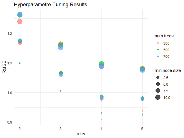
🍩 Bonus: Hyperparametre Tuning

ส่งท้าย เรามาดูวิธีใช้ tidymodels เพื่อทำ hyperparametre tuning ใน 5 ขั้นตอนกัน:

Prepare
Tune
Select
Fit
Evaluate

1️⃣ Prepare

ในการทำ hyperparametre tuning เราสามารถเขียนได้ทั้งแบบ standard flow และ workflow

ในบทความนี้ เราจะดูวิธีทำแบบ workflow ซึ่งเป็นวิธีที่ง่ายกว่ากัน

ในขั้นแรก เราต้องเตรียมของสำหรับ hyperparametre tuning 4 ข้อ ได้แก่:

No.	Input	Description
1	object	`workflow` object ที่รวม recipe และ model เอาไว้
2	resamples	การแบ่ง training set เพื่อทดสอบ hyperparametres
3	grid	การจับคู่ hyperparametres
4	metrics	ตัวชี้วัดที่ต้องการใช้ประเมิน hyperparametres

ข้อที่ 1. เตรียม object

เราเริ่มจากแบ่งข้อมูล:

# Set seed for reproducibility
set.seed(2025)

# Define the training set index
bt_split <- initial_split(data = bt,
                          prop = 0.8,
                          strata = medv)

# Create the training set
bt_train <- training(bt_split)

สร้าง recipe:

# Create a recipe
rec <- recipe(medv ~ .,
              data = bt_train) |>
  
  ## Remove near-zero variance predictors
  step_nzv(all_numeric_predictors()) |>
  
  ## Handle multicollinearity
  step_corr(all_numeric_predictors(),
            threshold = 0.8)

จากนั้น เรียกใช้ model โดยเราจะต้องกำหนด hyperparametre ที่ต้องการปรับ ด้วย tune():

# Define the tuning parameters
dt_model_tune <- decision_tree(cost_complexity = tune(),
                               tree_depth = tune(),
                               min_n = tune()) |>
  
  ## Set engine
  set_engine("rpart") |>
  
  ## Set mode
  set_mode("regression")

สุดท้าย เรารวม recipe และ model ไว้ใน workflow object:

# Define the workflow with tuning
bt_wfl_tune <- workflow() |>
  
  ## Add recipe
  add_recipe(rec) |>
  
  ## Add model
  add_model(dt_model_tune)

ข้อที่ 2. Resamples ซึ่งในที่นี้ เราจะใช้ k-fold cross-validation ที่แบ่ง training set ออกเป็น 5 ส่วน (4 ส่วนเพื่อ train และ 1 ส่วนเพื่อ test) แบบนี้:

# Set k-fold cross-validation for tuning
hpt_cv <- vfold_cv(bt_train,
                   v = 5,
                   strata = medv)

ข้อที่ 3. Grid ซึ่งเราจะใช้การจับคู่แบบสุ่มผ่าน grid_random():

# Set seed for reproducibility
set.seed(2025)

# Define the grid for tuning
hpt_grid <- grid_random(cost_complexity(range = c(-5, 0), trans = log10_trans()),
                        tree_depth(range = c(1, 20)),
                        min_n(range = c(2, 50)),
                        size = 20)

ข้อที่ 4. Metrics ซึ่งเราต้องเก็บไว้ใน metric_set():

# Define metrics
hpt_metrics = metric_set(mae,
                         rmse)

2️⃣ Tune

หลังจากเตรียม input ครบแล้ว เราสามารถ tune model ได้ด้วย tune_grid():

# Tune the model
dt_tune_results <- tune_grid(bt_wfl_tune,
                             resamples = hpt_cv,
                             grid = hpt_grid,
                             metrics = hpt_metrics)

3️⃣ Select

หลังจาก tune แล้ว เราสามารถดูค่า hyperparametres ที่ดีที่สุดตามตัวบ่งชี้ที่เราเลือกได้ด้วย show_best()

โดยในตัวอย่าง เราจะลองเลือก hyperparametres ที่ดีที่สุด 5 ชุดแรก โดยดูจาก RMSE:

# Show the best model
show_best(dt_tune_results,
          metric = "rmse",
          n = 5)

ผลลัพธ์:

# A tibble: 5 × 9
  cost_complexity tree_depth min_n .metric .estimator  mean     n
            <dbl>      <int> <int> <chr>   <chr>      <dbl> <int>
1       0.00311            3     5 rmse    standard    4.55     5
2       0.0167            16    12 rmse    standard    4.70     5
3       0.00150            5    28 rmse    standard    4.75     5
4       0.0000436         18    14 rmse    standard    4.88     5
5       0.0000345         11    39 rmse    standard    4.88     5
# ℹ 2 more variables: std_err <dbl>, .config <chr>

จากนั้น เราสามารถเลือกค่า hyperparametres ที่ดีที่สุดได้ด้วย select_best():

# Select the best model
dt_best_params <- select_best(dt_tune_results,
                              metric = "rmse")

4️⃣ Fit

ในขั้นที่ 4 เราจะใส่ค่า hyperparametres ที่เลือกมาเข้าไปใน workflow object ผ่าน finalize_workflow():

# Finalise the best workflow
dt_wkl_best <- finalize_workflow(bt_wfl_tune,
                                 dt_best_params)

จากนั้น train model ด้วย last_fit():

# Fit the best model
dt_best_fit <- last_fit(dt_wkl_best,
                        split = bt_split,
                        metrics = metric_set(mae, rmse))

5️⃣ Evaluate

สุดท้าย เราจะทดสอบ model ด้วย collect_predictions() และ collect_metrics():

# Collect predictions
predictions_best <- collect_predictions(dt_best_fit)

# Print predictions
predictions_best

ผลลัพธ์:

# A tibble: 103 × 5
   .pred id                .row  medv .config             
   <dbl> <chr>            <int> <dbl> <chr>               
 1  32.3 train/test split     3  34.7 Preprocessor1_Model1
 2  32.3 train/test split     4  33.4 Preprocessor1_Model1
 3  11.8 train/test split     9  16.5 Preprocessor1_Model1
 4  17.2 train/test split    25  15.6 Preprocessor1_Model1
 5  22.6 train/test split    40  30.8 Preprocessor1_Model1
 6  22.6 train/test split    53  25   Preprocessor1_Model1
 7  32.3 train/test split    56  35.4 Preprocessor1_Model1
 8  22.6 train/test split    79  21.2 Preprocessor1_Model1
 9  22.6 train/test split    82  23.9 Preprocessor1_Model1
10  34.5 train/test split    99  43.8 Preprocessor1_Model1
# ℹ 93 more rows
# ℹ Use `print(n = ...)` to see more rows

และ

# Collect metrics
metrics_best <- collect_metrics(dt_best_fit)

# Print metrics
metrics_best

ผลลัพธ์:

# A tibble: 2 × 4
  .metric .estimator .estimate .config             
  <chr>   <chr>          <dbl> <chr>               
1 mae     standard        3.48 Preprocessor1_Model1
2 rmse    standard        4.68 Preprocessor1_Model1

จะเห็นว่า hyperparametre tuning ทำให้ model ของเรามีประสิทธิภาพมากขึ้น เพราะมี MAE (3.70 vs 3.48) และ RMSE (5.13 vs 4.68) ที่ลดลง

😎 Summary

ในบทความนี้ เราได้ดูวิธีสร้าง ประเมิน และปรับ ML model ด้วย tidymodels ซึ่ง functions ต่าง ๆ ที่เราได้เรียนรู้สรุปตาม ML phase ได้ดังนี้:

Pre-processing:

Function	Description
`initial_split()`	แบ่งข้อมูล
`training()`	สร้าง training set
`testing()`	สร้าง test set
`recipe()`	กำหนดตัวแปรต้น ตัวแปรตาม
`step_*()`	กำหนดขั้นการแปลงข้อมูล
`prep()`	เตรียม recipe
`bake()`	เตรียมข้อมูล

Modelling:

Function	Description
`decision_tree()`	สร้าง decision tree
`set_engine()`	เรียกใช้ ML engine
`set_mode()`	กำหนดประเภท model
`fit()`	train model
`last_fit()`	train, ทำนาย, และประเมิน model

Post-processing:

Function	Description
`mae()`	คำนวณ MAE
`rmse()`	คำนวณ RMSE
`metric_set()`	กำหนดชุดตัวชี้วัด
`collect_predictions()`	เรียกดูคำทำนาย
`collect_metrics()`	เรียกดูตัวชี้วัด
`tune()`	กำหนด hyperparametres ที่ต้องการ tune
`vfold_cv()`	สร้าง k-fold cross-validation
`grid_random()`	สุ่มสร้างค่า hyperparametres ที่ต้องการทดสอบ
`tune_grid()`	tune model

All:

Function	Description
`workflow()`	รวม recipe และ model ไว้ด้วยกัน

📚 Further Reading

สำหรับคนที่สนใจ สามารถศึกษาเกี่ยวกับ tidymodels เพิ่มเติมได้ที่:

💪 Example Project

ดูตัวอย่างการใช้งาน tidymodels เพื่อสำหรับ data analytics project ได้ที่ Exploring & Predicting Employee Attrition With Machine Learning in R

😺 GitHub

ดู code ทั้งหมดในบทความนี้ได้ที่ GitHub:

📃 References

✅ R Book for Psychologists: หนังสือภาษา R สำหรับนักจิตวิทยา

📕 ขอฝากหนังสือเล่มแรกในชีวิตด้วยนะครับ 😆

🙋 ใครที่กำลังเรียนจิตวิทยาหรือทำงานสายจิตวิทยา และเบื่อที่ต้องใช้ software ราคาแพงอย่าง SPSS และ Excel เพื่อทำข้อมูล

💪 ผมขอแนะนำ R Book for Psychologists หนังสือสอนใช้ภาษา R เพื่อการวิเคราะห์ข้อมูลทางจิตวิทยา ที่เขียนมาเพื่อนักจิตวิทยาที่ไม่เคยมีประสบการณ์เขียน code มาก่อน

ในหนังสือ เราจะปูพื้นฐานภาษา R และพาไปดูวิธีวิเคราะห์สถิติที่ใช้บ่อยกัน เช่น:

Correlation
t-tests
ANOVA
Reliability
Factor analysis

🚀 เมื่ออ่านและทำตามตัวอย่างใน R Book for Psychologists ทุกคนจะไม่ต้องพึง SPSS และ Excel ในการทำงานอีกต่อไป และสามารถวิเคราะห์ข้อมูลด้วยตัวเองได้ด้วยความมั่นใจ

แล้วทุกคนจะแปลกใจว่า ทำไมภาษา R ง่ายขนาดนี้ 🙂‍↕️

👉 สนใจดูรายละเอียดหนังสือได้ที่ meb:

ดูรายละเอียดหนังสือ R Book for Psychologists

2025-06-19

สอนปลูกต้นไม้ในภาษา R (ภาค 2): วิธีสร้าง ประเมิน และปรับทูน random forest model ด้วย ranger package – ตัวอย่างการทำนายระดับการกินน้ำมันของรถใน mpg dataset

ในบทความนี้ เราจะไปทำความรู้จักกับ random forest รวมทั้งการสร้าง ประเมิน และปรับทูน random forest model ด้วย ranger package ในภาษา R

ถ้าพร้อมแล้ว ไปเริ่มกันเลย

🌲 Random Forest Model คืออะไร?

Random forest model เป็น tree-based model ซึ่งสุ่มสร้าง decision trees ขึ้นมาหลาย ๆ ต้น (forest) และใช้ผลลัพธ์ในภาพรวมเพื่อทำนายข้อมูลสุดท้าย:

Regression task: หาค่าเฉลี่ยของผลลัพธ์จากทุกต้น
Classification task: ดูผลลัพธ์ที่เป็นเสียงโหวตข้างมาก

Random forest เป็น model ที่ทรงพลัง เพราะใช้ผลรวมของหลาย ๆ decision trees แม้ว่า decision tree แต่ละต้นจะมีความสามารถในการทำนายนอยก็ตาม

💻 Random Forest Models ในภาษา R

ในภาษา R เรามี 2 packages ที่นิยมใช้สร้าง random forest model ได้แก่:

randomForest ซึ่งเป็น package ที่มีลูกเล่น แต่เก่ากว่า
ranger ซึ่งใหม่กว่า ประมวลผลได้เร็วกว่า และใช้งานง่ายกว่า

ในบทความก่อน เราดูวิธีการใช้ randomForest แล้ว

ในบทความนี้ เราจะไปดูวิธีใช้ ranger โดยใช้ mpg dataset เป็นตัวอย่างกัน

🚗 mpg Dataset

mpg dataset เป็น dataset จาก ggplots2 package และมีข้อมูลของรถ 38 รุ่น จากช่วงปี ช่วง ค.ศ. 1999 ถึง 2008 ทั้งหมด 11 columns ดังนี้:

No.	Column	Description
1	`manufacturer`	ผู้ผลิต
2	`model`	รุ่นรถ
3	`displ`	ขนาดถังน้ำมัน (ลิตร)
4	`year`	ปีที่ผลิต
5	`cyl`	จำนวนลูกสูบ
6	`trans`	ประเภทเกียร์
7	`drv`	ประเภทล้อขับเคลื่อน
8	`cty`	ระดับการกินน้ำมันเวลาวิ่งในเมือง
9	`hwy`	ระดับการกินน้ำมันเวลาวิ่งบน highway
10	`fl`	ประเภทน้ำมัน
11	`class`	ประเภทรถ

ในบทความนี้ เราจะลองใช้ ranger เพื่อทำนาย hwy กัน

เราสามารถเตรียม mpg เพื่อสร้าง random forest model ได้ดังนี้

โหลด dataset:

# Install ggplot2
install.packages("ggplot2")

# Load ggplot2
library(ggplot2)

# Load the dataset
data(mpg)

ดูตัวอย่าง dataset:

# Preview
head(mpg)

ผลลัพธ์:

# A tibble: 6 × 11
  manufacturer model displ  year   cyl trans      drv     cty   hwy fl    class  
  <chr>        <chr> <dbl> <int> <int> <chr>      <chr> <int> <int> <chr> <chr>  
1 audi         a4      1.8  1999     4 auto(l5)   f        18    29 p     compact
2 audi         a4      1.8  1999     4 manual(m5) f        21    29 p     compact
3 audi         a4      2    2008     4 manual(m6) f        20    31 p     compact
4 audi         a4      2    2008     4 auto(av)   f        21    30 p     compact
5 audi         a4      2.8  1999     6 auto(l5)   f        16    26 p     compact
6 audi         a4      2.8  1999     6 manual(m5) f        18    26 p     compact

สำรวจโครงสร้าง:

# View the structure
str(mpg)

ผลลัพธ์:

tibble [234 × 11] (S3: tbl_df/tbl/data.frame)
 $ manufacturer: chr [1:234] "audi" "audi" "audi" "audi" ...
 $ model       : chr [1:234] "a4" "a4" "a4" "a4" ...
 $ displ       : num [1:234] 1.8 1.8 2 2 2.8 2.8 3.1 1.8 1.8 2 ...
 $ year        : int [1:234] 1999 1999 2008 2008 1999 1999 2008 1999 1999 2008 ...
 $ cyl         : int [1:234] 4 4 4 4 6 6 6 4 4 4 ...
 $ trans       : chr [1:234] "auto(l5)" "manual(m5)" "manual(m6)" "auto(av)" ...
 $ drv         : chr [1:234] "f" "f" "f" "f" ...
 $ cty         : int [1:234] 18 21 20 21 16 18 18 18 16 20 ...
 $ hwy         : int [1:234] 29 29 31 30 26 26 27 26 25 28 ...
 $ fl          : chr [1:234] "p" "p" "p" "p" ...
 $ class       : chr [1:234] "compact" "compact" "compact" "compact" ...

จากผลลัพธ์จะเห็นว่า บาง columns (เช่น manufacturer, model) มีข้อมูลประเภท character ซึ่งเราควระเปลี่ยนเป็น factor เพื่อช่วยให้การสร้าง model มีประสิทธิภาพมากขึ้น:

# Convert character columns to factor

## Get character columns
chr_cols <- c("manufacturer", "model",
              "trans", "drv",
              "fl", "class")

## For-loop through the character columns
for (col in chr_cols) {
  mpg[[col]] <- as.factor(mpg[[col]])
}

## Check the results
str(mpg)

ผลลัพธ์:

tibble [234 × 11] (S3: tbl_df/tbl/data.frame)
 $ manufacturer: Factor w/ 15 levels "audi","chevrolet",..: 1 1 1 1 1 1 1 1 1 1 ...
 $ model       : Factor w/ 38 levels "4runner 4wd",..: 2 2 2 2 2 2 2 3 3 3 ...
 $ displ       : num [1:234] 1.8 1.8 2 2 2.8 2.8 3.1 1.8 1.8 2 ...
 $ year        : int [1:234] 1999 1999 2008 2008 1999 1999 2008 1999 1999 2008 ...
 $ cyl         : int [1:234] 4 4 4 4 6 6 6 4 4 4 ...
 $ trans       : Factor w/ 10 levels "auto(av)","auto(l3)",..: 4 9 10 1 4 9 1 9 4 10 ...
 $ drv         : Factor w/ 3 levels "4","f","r": 2 2 2 2 2 2 2 1 1 1 ...
 $ cty         : int [1:234] 18 21 20 21 16 18 18 18 16 20 ...
 $ hwy         : int [1:234] 29 29 31 30 26 26 27 26 25 28 ...
 $ fl          : Factor w/ 5 levels "c","d","e","p",..: 4 4 4 4 4 4 4 4 4 4 ...
 $ class       : Factor w/ 7 levels "2seater","compact",..: 2 2 2 2 2 2 2 2 2 2 ...

ตอนนี้ เราพร้อมที่จะนำ dataset ไปใช้งานกับ ranger แล้ว

🐣 ranger Basics

การใช้งาน ranger มีอยู่ 4 ขั้นตอน:

ติดตั้งและโหลด ranger
สร้าง training และ test sets
สร้าง random forest model
ทดสอบความสามารถของ model

1️⃣ ติดตั้งและโหลด ranger

ในครั้งแรกสุด ให้เราติดตั้ง ranger ด้วยคำสั่ง install.packages():

# Install
install.packages("ranger")

และทุกครั้งที่เราต้องการใช้งาน ranger ให้เราเรียกใช้งานด้วย library():

# Load
library(ranger)

2️⃣ สร้าง Training และ Test Sets

ในขั้นที่ 2 เราจะแบ่ง dataset เป็น 2 ส่วน ได้แก่:

Training set สำหรับสร้าง model (70% ของ dataset)
Test set สำหรับทดสอบ model (30% ของ dataset)

# Split the data

## Set seed for reproducibility
set.seed(123)

## Get training rows
train_rows <- sample(nrow(mpg),
                     nrow(mpg) * 0.7)

## Create a training set
train <- mpg[train_rows, ]

## Create a test set
test <- mpg[-train_rows, ]

3️⃣ สร้าง Random Forest Model

ในขั้นที่ 3 เราจะสร้าง random forest ด้วย ranger() ซึ่งต้องการ input หลัก 2 อย่าง ดังนี้:

ranger(formula, data)

formula: ระบุตัวแปรต้นและตัวแปรตามที่ใช้ในการสร้าง model
data: dataset ที่ใช้สร้าง model (เราจะใช้ training set กัน)

เราจะเรียกใช้ ranger() ดังนี้:

# Initial random forest model

## Set seed for reproducibility
set.seed(123)

## Train the model
rf_model <- ranger(hwy ~ .,
                   data = train)

Note: เราใช้ set.seed() เพื่อให้เราสามารถสร้าง model ซ้ำได้ เพราะ random forest มีการสร้าง decision trees แบบสุ่ม

เมื่อได้ model มาแล้ว เราสามารถดูรายละเอียดของ model ได้แบบนี้:

# Print the model
rf_model

ผลลัพธ์:

Ranger result

Call:
 ranger(hwy ~ ., data = train) 

Type:                             Regression 
Number of trees:                  500 
Sample size:                      163 
Number of independent variables:  10 
Mtry:                             3 
Target node size:                 5 
Variable importance mode:         none 
Splitrule:                        variance 
OOB prediction error (MSE):       1.682456 
R squared (OOB):                  0.9584596

ในผลลัพธ์ เราจะเห็นลักษณะต่าง ๆ ของ model เช่น ประเภท model (type) และ จำนวน decision trees ที่ถูกสร้างขึ้นมา (sample size)

4️⃣ ทดสอบความสามารถของ Model

สุดท้าย เราจะทดสอบความสามารถของ model ในการทำนายข้อมูล โดยเริ่มจากใช้ model ทำนายข้อมูลใน test set:

# Make predictions
preds <- predict(rf_model,
                 data = test)$predictions

จากนั้น คำนวณตัวบ่งชี้ความสามารถ (metric) ซึ่งสำหรับ regression model มีอยู่ 3 ตัว ได้แก่:

MAE (mean absolute error): ค่าเฉลี่ยความคลาดเคลื่อนแบบสัมบูรณ์ (ยิ่งน้อยยิ่งดี)
RMSE (root mean square error): ค่าเฉลี่ยความคาดเคลื่อนแบบยกกำลังสอง (ยิ่งน้อยยิ่งดี)
R squared: สัดส่วนข้อมูลที่อธิบายได้ด้วย model (ยิ่งมากยิ่งดี)

# Get errors
errors <- test$hwy - preds

# Calculate MAE
mae <- mean(abs(errors))

# Calculate RMSE
rmse <- sqrt(mean(errors^2))

# Calculate R squared
r_sq <- 1 - (sum((errors)^2) / sum((test$hwy - mean(test$hwy))^2))

# Print the results
cat("Initial model MAE:", round(mae, 2), "\n")
cat("Initial model RMSE:", round(rmse, 2), "\n")
cat("Initial model R squared:", round(r_sq, 2), "\n")

ผลลัพธ์:

Initial model MAE: 0.79
Initial model RMSE: 1.07
Initial model R squared: 0.95

⏲️ Hyperparametre Tuning

ranger มี hyperparametre มากมายที่เราสามารถปรับแต่งเพื่อเพิ่มประสิทธิภาพของ random forest model ได้ เช่น:

num.trees: จำนวน decision trees ที่จะสร้าง
mtry: จำนวนตัวแปรต้นที่จะถูกสุ่มไปใช้ในแต่ละ node
min.node.size: จำนวนข้อมูลขั้นต่ำที่แต่ละ node จะต้องมี

เราสามารถใช้ for loop เพื่อปรับหาค่า hyperparametre ที่ดีที่สุดได้ดังนี้:

# Define hyperparametres
ntree_vals <- c(300, 500, 700)
mtry_vals <- 2:5
min_node_vals <- c(1, 5, 10)

# Create a hyperparametre grid
grid <- expand.grid(num.trees = ntree_vals,
                    mtry = mtry_vals,
                    min.node.size = min_node_vals)

# Instantiate an empty data frame
hpt_results <- data.frame()

# For-loop through the hyperparametre grid
for (i in 1:nrow(grid)) {
  
  ## Get the combination
  params <- grid[i, ]
  
  ## Set seed for reproducibility
  set.seed(123)
  
  ## Fit the model
  model <- ranger(hwy ~ .,
                  data = train,
                  num.trees = params$num.trees,
                  mtry = params$mtry,
                  min.node.size = params$min.node.size)
  
  ## Make predictions
  preds <- predict(model,
                   data = test)$predictions
  
  ## Get errors
  errors <- test$hwy - preds
  
  ## Calculate MAE
  mae <- mean(abs(errors))
  
  ## Calculate RMSE
  rmse <- sqrt(mean(errors^2))
  
  ## Store the results
  hpt_results <- rbind(hpt_results,
                       cbind(params,
                             MAE = mae,
                             RMSE = rmse))
}

# View the results
hpt_results

ผลลัพธ์:

   num.trees mtry min.node.size       MAE      RMSE
1        300    2             1 0.8101026 1.0971836
2        500    2             1 0.8012484 1.0973957
3        700    2             1 0.8039271 1.1001252
4        300    3             1 0.7434543 1.0051344
5        500    3             1 0.7417985 1.0069989
6        700    3             1 0.7421666 1.0028184
7        300    4             1 0.6989314 0.9074216
8        500    4             1 0.7130704 0.9314843
9        700    4             1 0.7141147 0.9292718
10       300    5             1 0.7157657 0.9370918
11       500    5             1 0.7131899 0.9266787
12       700    5             1 0.7091556 0.9238312
13       300    2             5 0.8570125 1.1673637
14       500    2             5 0.8515116 1.1736009
15       700    2             5 0.8522571 1.1756648
16       300    3             5 0.7885005 1.0654548
17       500    3             5 0.7872713 1.0664734
18       700    3             5 0.7859149 1.0581331
19       300    4             5 0.7561500 0.9790160
20       500    4             5 0.7623437 0.9869463
21       700    4             5 0.7611660 0.9813048
22       300    5             5 0.7615190 0.9777769
23       500    5             5 0.7615861 0.9804616
24       700    5             5 0.7613151 0.9788333
25       300    2            10 0.9257704 1.2391377
26       500    2            10 0.9292344 1.2611164
27       700    2            10 0.9258555 1.2635794
28       300    3            10 0.8790601 1.1635695
29       500    3            10 0.8704461 1.1594165
30       700    3            10 0.8704562 1.1507016
31       300    4            10 0.8609516 1.0887466
32       500    4            10 0.8672105 1.0962367
33       700    4            10 0.8624934 1.0875710
34       300    5            10 0.8558867 1.0811168
35       500    5            10 0.8567463 1.0783473
36       700    5            10 0.8536824 1.0751511

จะเห็นว่า เราจะได้ MSE และ RMSE ของส่วนผสมระหว่างแต่ละ hyperparametre มา

เราสามารถใช้ ggplot() เพื่อช่วยเลือก hyperparametres ที่ดีที่สุดได้ดังนี้:

# Visualise the results
ggplot(hpt_results,
       aes(x = mtry,
           y = RMSE,
           color = factor(num.trees))) +
  
  ## Use scatter plot
  geom_point(aes(size = min.node.size)) +
  
  ## Set theme to minimal
  theme_minimal() +
  
  ## Add title, labels, and legends
  labs(title = "Hyperparametre Tuning Results",
       x = "mtry",
       y = "RMSE",
       color = "num.trees",
       size = "min.node.size")

ผลลัพธ์:

จากกราฟ จะเห็นได้ว่า hyperparametres ที่ดีที่สุด (มี RMSE น้อยที่สุด) คือ:

num.trees = 300
mtry = 4
min.node.size = 2.5

เมื่อได้ค่า hyperparametres แล้ว เราสามารถใส่ค่าเหล่านี้กลับเข้าไปใน model และทดสอบความสามารถได้เลย

สร้าง model:

# Define the best hyperparametres
best_num.tree <- 300
best_mtry <- 4
best_min.node.size <- 2.5

# Fit the model
rf_model_new <- ranger(hwy ~ .,
                       data = train,
                       num.tree = best_num.tree,
                       mtry = best_mtry,
                       min.node.size = best_min.node.size)

ทดสอบความสามารถ:

# Evaluate the model

## Make predictions
preds_new <- predict(rf_model_new,
                     data = test)$predictions

## Get errors
errors_new <- test$hwy - preds_new

## Calculate MAE
mae_new <- mean(abs(errors_new))

## Calculate RMSE
rmse_new <- sqrt(mean(errors_new^2))

## Calculate R squared
r_sq_new <- 1 - (sum((errors_new)^2) / sum((test$hwy - mean(test$hwy))^2))

## Print the results
cat("Final model MAE:", round(mae_new, 2), "\n")
cat("Final model RMSE:", round(rmse_new, 2), "\n")
cat("Final model R squared:", round(r_sq_new, 2), "\n")

ผลลัพธ์:

Final model MAE: 0.71
Final model RMSE: 0.93
Final model R squared: 0.96

เราสามารถเปรียบเทียบความสามารถของ model ล่าสุด (final model) กับ model ก่อนหน้านี้ (initial model) ได้:

# Compare the two models
model_comp <- data.frame(Model = c("Initial", "Final"),
                         MAE = c(round(mae, 2), round(mae_new, 2)),
                         RMSE = c(round(rmse, 2), round(rmse_new, 2)),
                         R_Squared = c(round(r_sq, 2), round(r_sq_new, 2)))

# Print
model_comp

ผลลัพธ์:

    Model  MAE RMSE R_Squared
1 Initial 0.85 1.08      0.95
2   Final 0.71 0.93      0.96

ซึ่งจะเห็นว่า model ใหม่สามารถทำนายข้อมูลได้ดีขึ้น เพราะมี MAE และ RMSE ที่ลดลง รวมทั้ง R squared ที่เพิ่มขึ้น

🍩 Bonus: Variable Importance

ส่งท้าย ในกรณีที่เราต้องการดูว่า ตัวแปรต้นไหนมีความสำคัญต่อการทำนายมากที่สุด เราสามารถใช้ importance argument ใน ranger() คู่กับ vip() จาก vip package ได้แบบนี้:

# Fit the model with importance
rf_model_new <- ranger(hwy ~ .,
                       data = train,
                       num.tree = best_num.tree,
                       mtry = best_mtry,
                       min.node.size = best_min.node.size,
                       importance = "permutation") # Add importance

# Install vip package
install.packages("vip")

# Load vip package
library(vip)

# Get variabe importance
vip(rf_model_new)  +
  
  ## Add title and labels
  labs(title = "Variable Importance - Final Random Forest Model",
       x = "Variables",
       y = "Importance") +
  
  ## Set theme to minimal
  theme_minimal()

ผลลัพธ์:

จากกราฟ จะเห็นได้ว่า ตัวแปรต้นที่สำคัญที่สุด 3 ตัว ได้แก่:

cty: ระดับการกินน้ำมันเวลาวิ่งในเมือง
displ: ขนาดถังน้ำมัน (ลิตร)
cyl: จำนวนลูกสูบ

😎 Summary

ในบทความนี้ เราได้ดูวิธีการใช้ ranger package เพื่อ:

สร้าง random forest model
ปรับทูน model

พร้อมวิธีการประเมิน model ด้วย predict() และการคำนวณ MAE, RMSE, และ R squared รวมทั้งดูความสำคัญของตัวแปรต้นด้วย vip package

😺 GitHub

ดู code ทั้งหมดในบทความนี้ได้ที่ GitHub

📃 References

✅ R Book for Psychologists: หนังสือภาษา R สำหรับนักจิตวิทยา

📕 ขอฝากหนังสือเล่มแรกในชีวิตด้วยนะครับ 😆

Correlation
t-tests
ANOVA
Reliability
Factor analysis

แล้วทุกคนจะแปลกใจว่า ทำไมภาษา R ง่ายขนาดนี้ 🙂‍↕️

👉 สนใจดูรายละเอียดหนังสือได้ที่ meb:

ดูรายละเอียดหนังสือ R Book for Psychologists

2025-06-05

Tag: Hyperparametre tuning

🔢 Dataset

🏠 Boston

⬇️ Get Boston

🧹 Prepare Boston

🛩️ tidymodels

🏁 Getting Started

🌊 Flows

🥐 Method #1. Standard Flow

1️⃣ Split the Data

2️⃣ Create a Recipe

3️⃣ Prep & Bake

4️⃣ Instantiate a Model

5️⃣ Fit the Model

6️⃣ Make Predictions

7️⃣ Evaluate the Model

🍰 Method #2. Workflow

1️⃣ Split the Data

2️⃣ Create a Recipe

3️⃣ Instantiate the Model

4️⃣ Bundle the Recipe and the Model

5️⃣ Fit the Model

6️⃣ Evaluate the Model

🍩 Bonus: Hyperparametre Tuning

1️⃣ Prepare

2️⃣ Tune

3️⃣ Select

4️⃣ Fit

5️⃣ Evaluate

😎 Summary

📚 Further Reading

💪 Example Project

😺 GitHub

📃 References

✅ R Book for Psychologists: หนังสือภาษา R สำหรับนักจิตวิทยา

Share this:

🌲 Random Forest Model คืออะไร?

💻 Random Forest Models ในภาษา R

🚗 mpg Dataset

🐣 ranger Basics

1️⃣ ติดตั้งและโหลด ranger

2️⃣ สร้าง Training และ Test Sets

3️⃣ สร้าง Random Forest Model

4️⃣ ทดสอบความสามารถของ Model

⏲️ Hyperparametre Tuning

🍩 Bonus: Variable Importance

😎 Summary

😺 GitHub

📃 References

✅ R Book for Psychologists: หนังสือภาษา R สำหรับนักจิตวิทยา

Share this: