Data frame เป็นหนึ่งใน data structure ที่พบบ่อยที่สุดในการทำงานกับข้อมูล
Data frame เก็บข้อมูลในรูปแบบตาราง โดย:
- 1 row = 1 รายการ (เช่น ข้อมูลของ John)
- 1 column = 1 ประเภทข้อมูล (เช่น อายุ)
ตัวอย่าง data frame:
ในบทความนี้ เราจะมาสรุป 10 วิธีในการทำงานกับ data frame กัน:
- Creating: การสร้าง data frame
- Previewing: การดูข้อมูล data frame
- Indexing: การเลือก columns ที่ต้องการ
- Subsetting: การเลือก rows และ columns ที่ต้องการ
- Filtering: การกรองข้อมูล
- Sorting: การจัดลำดับข้อมูล
- Aggregating: การสรุปข้อมูล
- Adding columns: การเพิ่ม columns ใหม่
- Removing columns: การลบ columns
- Binding: การเชื่อมข้อมูลใหม่เข้ากับ data frame
ถ้าพร้อมแล้ว ไปเริ่มกันเลย
- 1️⃣ Creating
- 2️⃣ Previewing
- 3️⃣ Indexing
- 4️⃣ Subsetting
- 5️⃣ Filtering
- 6️⃣ Sorting
- 7️⃣ Aggregating
- 8️⃣ Adding Columns
- 9️⃣ Removing Columns
- 🔟 Binding
- 😺 GitHub
- 📃 References
- ✅ R Book for Psychologists: หนังสือภาษา R สำหรับนักจิตวิทยา
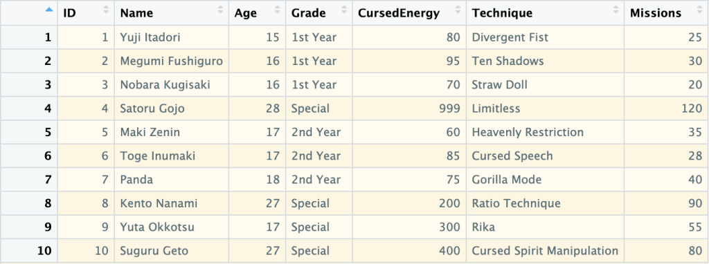
1️⃣ Creating

เราสามารถสร้าง data frame ด้วย data.frame() ซึ่งต้องการ ชื่อ column และ vector ที่เก็บข้อมูลของ column นั้น ๆ:
# Create a data frame
jjk_df <- data.frame(
  ID = 1:10,
  Name = c("Yuji Itadori", "Megumi Fushiguro", "Nobara Kugisaki", "Satoru Gojo",
           "Maki Zenin", "Toge Inumaki", "Panda", "Kento Nanami", "Yuta Okkotsu", "Suguru Geto"),
  Age = c(15, 16, 16, 28, 17, 17, 18, 27, 17, 27),
  Grade = c("1st Year", "1st Year", "1st Year", "Special", "2nd Year",
            "2nd Year", "2nd Year", "Special", "Special", "Special"),
  CursedEnergy = c(80, 95, 70, 999, 60, 85, 75, 200, 300, 400),
  Technique = c("Divergent Fist", "Ten Shadows", "Straw Doll", "Limitless",
                "Heavenly Restriction", "Cursed Speech", "Gorilla Mode",
                "Ratio Technique", "Rika", "Cursed Spirit Manipulation"),
  Missions = c(25, 30, 20, 120, 35, 28, 40, 90, 55, 80)
)

# View the result
jjk_df
ผลลัพธ์:
   ID             Name Age    Grade CursedEnergy                  Technique Missions
1   1     Yuji Itadori  15 1st Year           80             Divergent Fist       25
2   2 Megumi Fushiguro  16 1st Year           95                Ten Shadows       30
3   3  Nobara Kugisaki  16 1st Year           70                 Straw Doll       20
4   4      Satoru Gojo  28  Special          999                  Limitless      120
5   5       Maki Zenin  17 2nd Year           60       Heavenly Restriction       35
6   6     Toge Inumaki  17 2nd Year           85              Cursed Speech       28
7   7            Panda  18 2nd Year           75               Gorilla Mode       40
8   8     Kento Nanami  27  Special          200            Ratio Technique       90
9   9     Yuta Okkotsu  17  Special          300                       Rika       55
10 10      Suguru Geto  27  Special          400 Cursed Spirit Manipulation       80
2️⃣ Previewing
เรามี 8 functions สำหรับดูข้อมูล data frame:
| No. | Function | For |
|---|---|---|
| 1 | View() | ดูข้อมูลทั้งหมด |
| 2 | head() | ดูข้อมูล 6 rows แรก |
| 3 | tail() | ดูข้อมูล 6 rows สุดท้าย |
| 4 | str() | ดูโครงสร้างข้อมูล |
| 5 | summary() | ดูสถิติข้อมูล |
| 6 | dim() | ดูจำนวน rows และ columns |
| 7 | nrow() | ดูจำนวน rows |
| 8 | ncol() | ดูจำนวน columns |
เราไปดูตัวอย่างทั้ง 8 functions กัน
.
👀 View()
View() ใช้ดูข้อมูลทั้งหมดใน data frame:
# View the whole data frame
View(jjk_df)
เราจะเห็นผลลัพธ์ในหน้าต่างใหม่:
Note: เนื่องจาก View() แสดงข้อมูลทั้งหมด จึงเหมาะกับการใช้งานกับ data frame ขนาดเล็ก
.
🙊 head()
head() ใช้ดูข้อมูล 6 rows แรกใน data frame:
# View the first 6 rows
head(jjk_df)
ผลลัพธ์:
  ID             Name Age    Grade CursedEnergy            Technique Missions
1  1     Yuji Itadori  15 1st Year           80       Divergent Fist       25
2  2 Megumi Fushiguro  16 1st Year           95          Ten Shadows       30
3  3  Nobara Kugisaki  16 1st Year           70           Straw Doll       20
4  4      Satoru Gojo  28  Special          999            Limitless      120
5  5       Maki Zenin  17 2nd Year           60 Heavenly Restriction       35
6  6     Toge Inumaki  17 2nd Year           85        Cursed Speech       28
.
🐒 tail()
tail() ใช้ดูข้อมูล 6 rows สุดท้ายใน data frame:
# View the last 6 rows
tail(jjk_df)
ผลลัพธ์:
   ID         Name Age    Grade CursedEnergy                  Technique Missions
5   5   Maki Zenin  17 2nd Year           60       Heavenly Restriction       35
6   6 Toge Inumaki  17 2nd Year           85              Cursed Speech       28
7   7        Panda  18 2nd Year           75               Gorilla Mode       40
8   8 Kento Nanami  27  Special          200            Ratio Technique       90
9   9 Yuta Okkotsu  17  Special          300                       Rika       55
10 10  Suguru Geto  27  Special          400 Cursed Spirit Manipulation       80
.
🏗️ str()
str() ใช้ดูโครงสร้างข้อมูลของ data frame:
# View the data frame structure
str(jjk_df)
ผลลัพธ์:
'data.frame':	10 obs. of  7 variables:
 $ ID          : int  1 2 3 4 5 6 7 8 9 10
 $ Name        : chr  "Yuji Itadori" "Megumi Fushiguro" "Nobara Kugisaki" "Satoru Gojo" ...
 $ Age         : num  15 16 16 28 17 17 18 27 17 27
 $ Grade       : chr  "1st Year" "1st Year" "1st Year" "Special" ...
 $ CursedEnergy: num  80 95 70 999 60 85 75 200 300 400
 $ Technique   : chr  "Divergent Fist" "Ten Shadows" "Straw Doll" "Limitless" ...
 $ Missions    : num  25 30 20 120 35 28 40 90 55 80
จากผลลัพธ์ เราจะเห็นข้อมูล 5 อย่าง ได้แก่:
- จำนวน rows (
obs.) - จำนวน columns (
variables) - ชื่อ columns (เช่น
ID) - ประเภทข้อมูลของแต่ละ column (เช่น
int) - ตัวอย่างข้อมูลของแต่ละ column (เช่น
1 2 3 4 5 6 7 8 9 10)
.
🧮 summary()
summary() ใช้สรุปข้อมูลใน data frame เช่น:
- ค่าเฉลี่ย (
Mean) - จำนวนข้อมูล (
Length)
# View the summary
summary(jjk_df)
ผลลัพธ์:
       ID            Name                Age           Grade            CursedEnergy     Technique            Missions
 Min.   : 1.00   Length:10          Min.   :15.00   Length:10          Min.   : 60.00   Length:10          Min.   : 20.00
 1st Qu.: 3.25   Class :character   1st Qu.:16.25   Class :character   1st Qu.: 76.25   Class :character   1st Qu.: 28.50
 Median : 5.50   Mode  :character   Median :17.00   Mode  :character   Median : 90.00   Mode  :character   Median : 37.50
 Mean   : 5.50                      Mean   :19.80                      Mean   :236.40                      Mean   : 52.30
 3rd Qu.: 7.75                      3rd Qu.:24.75                      3rd Qu.:275.00                      3rd Qu.: 73.75
 Max.   :10.00                      Max.   :28.00                      Max.   :999.00                      Max.   :120.00
.
💠 dim()
dim() ใช้แสดงจำนวน rows และ columns ใน data frame:
# View the dimensions
dim(jjk_df)
ผลลัพธ์:
[1] 10 7
.
🚣 nrow()
nrow() ใช้แสดงจำนวน rows ใน data frame:
# Get the number of rows
nrow(jjk_df)
ผลลัพธ์:
[1] 10
.
🏦 ncol()
ncol() ใช้แสดงจำนวน columns ใน data frame:
# Get the number of columns
ncol(jjk_df)
ผลลัพธ์:
[1] 7
3️⃣ Indexing
Indexing หมายถึง การเลือก columns ที่ต้องการ ซึ่งเราทำได้ 2 วิธี:
- ใช้
$(นิยมใช้) - ใช้
[[]]
💰 Using $
เราสามารถใช้ $ ได้แบบนี้:
df$col
ยกตัวอย่างเช่น เลือก column Name:
# Index with $
jjk_df$Name
ผลลัพธ์:
 [1] "Yuji Itadori"     "Megumi Fushiguro" "Nobara Kugisaki"  "Satoru Gojo"      "Maki Zenin"
 [6] "Toge Inumaki"     "Panda"            "Kento Nanami"     "Yuta Okkotsu"     "Suguru Geto"
.
🔳 Using [[]]
เราสามารถใช้ [[]] ได้แบบนี้:
df[["col"]]
ยกตัวอย่างเช่น เลือก column Name:
# Index with [[]]
jjk_df[["Name"]]
ผลลัพธ์:
 [1] "Yuji Itadori"     "Megumi Fushiguro" "Nobara Kugisaki"  "Satoru Gojo"      "Maki Zenin"
 [6] "Toge Inumaki"     "Panda"            "Kento Nanami"     "Yuta Okkotsu"     "Suguru Geto"
4️⃣ Subsetting
Subsetting คือ การเลือก rows และ columns จาก data frame ซึ่งเราทำได้ 2 วิธี:
- ใช้
df[rows, cols]syntax - ใช้
subset()
.
🍽️ df[rows, cols]
เราสามารถใช้ df[rows, cols] ได้ 3 แบบ:
- เลือก rows
- เลือก columns
- เลือก rows และ columns
แบบที่ 1. เลือก rows อย่างเดียว:
# Subset rows only
jjk_df[1:5, ]
ผลลัพธ์:
  ID             Name Age    Grade CursedEnergy            Technique Missions
1  1     Yuji Itadori  15 1st Year           80       Divergent Fist       25
2  2 Megumi Fushiguro  16 1st Year           95          Ten Shadows       30
3  3  Nobara Kugisaki  16 1st Year           70           Straw Doll       20
4  4      Satoru Gojo  28  Special          999            Limitless      120
5  5       Maki Zenin  17 2nd Year           60 Heavenly Restriction       35
แบบที่ 2. เลือก columns อย่างเดียว:
# Subset columns only
jjk_df[, "Name"]
ผลลัพธ์:
 [1] "Yuji Itadori"     "Megumi Fushiguro" "Nobara Kugisaki"  "Satoru Gojo"      "Maki Zenin"
 [6] "Toge Inumaki"     "Panda"            "Kento Nanami"     "Yuta Okkotsu"     "Suguru Geto"
แบบที่ 3. เลือก rows และ columns:
# Subset rows and columns
jjk_df[1:5, c("Name", "Technique")]
ผลลัพธ์:
              Name            Technique
1     Yuji Itadori       Divergent Fist
2 Megumi Fushiguro          Ten Shadows
3  Nobara Kugisaki           Straw Doll
4      Satoru Gojo            Limitless
5       Maki Zenin Heavenly Restriction
.
🔪 subset()
เราสามารถ subset ข้อมูลได้ด้วย subset() ซึ่งต้องการ 2 arguments:
subset(x, select)
x= data frameselect= columns ที่ต้องการเลือก
# Subset using susbet() - select conlumns only
subset(jjk_df, select = c("Name", "Technique"))
ผลลัพธ์:
               Name                  Technique
1      Yuji Itadori             Divergent Fist
2  Megumi Fushiguro                Ten Shadows
3   Nobara Kugisaki                 Straw Doll
4       Satoru Gojo                  Limitless
5        Maki Zenin       Heavenly Restriction
6      Toge Inumaki              Cursed Speech
7             Panda               Gorilla Mode
8      Kento Nanami            Ratio Technique
9      Yuta Okkotsu                       Rika
10      Suguru Geto Cursed Spirit Manipulation
ในกรณีที่เราต้องการเลือก rows ด้วย เราจะต้องกำหนด rows ใน x:
# Subset using susbet() - select both rows and columns
subset(jjk_df[1:5, ], select = c("Name", "Technique"))
ผลลัพธ์:
              Name            Technique
1     Yuji Itadori       Divergent Fist
2 Megumi Fushiguro          Ten Shadows
3  Nobara Kugisaki           Straw Doll
4      Satoru Gojo            Limitless
5       Maki Zenin Heavenly Restriction
5️⃣ Filtering

เราสามารถกรองข้อมูลใน data frame ได้ 2 วิธี:
- ใช้
df[rows, cols]syntax - ใช้
subset()
.
🍽️ df[rows, cols]
เราสามารถกรองข้อมูลด้วย df[rows, cols] โดยกำหนดเงื่อนไขการกรองใน rows
เช่น กรองข้อมูลตัวละครที่อยู่ปี 1:
# Filter using df[rows, cols] - 1 condition
jjk_df[jjk_df$Grade == "1st Year", ]
ผลลัพธ์:
  ID             Name Age    Grade CursedEnergy      Technique Missions
1  1     Yuji Itadori  15 1st Year           80 Divergent Fist       25
2  2 Megumi Fushiguro  16 1st Year           95    Ten Shadows       30
3  3  Nobara Kugisaki  16 1st Year           70     Straw Doll       20
ในกรณีที่เรามีมากกว่า 1 เงื่อนไข เราสามารถใช้ logical operators ช่วยได้:
| Operator | Meaning |
|---|---|
& | AND |
| | OR |
! | NOT |
ยกตัวอย่างเช่น กรองข้อมูลตัวละครที่อยู่ปี 1 และมีอายุ 15 ปี:
# Filter using df[rows, cols] - multiple conditions
jjk_df[jjk_df$Grade == "1st Year" & jjk_df$Age == 15, ]
ผลลัพธ์:
  ID         Name Age    Grade CursedEnergy      Technique Missions
1  1 Yuji Itadori  15 1st Year           80 Divergent Fist       25
.
🔪 subset()
เราสามารถใช้ subset() เพื่อกรองข้อมูลได้แบบนี้:
# Filter using subset() - 1 condition
subset(jjk_df, Grade == "1st Year")
ผลลัพธ์:
  ID             Name Age    Grade CursedEnergy      Technique Missions
1  1     Yuji Itadori  15 1st Year           80 Divergent Fist       25
2  2 Megumi Fushiguro  16 1st Year           95    Ten Shadows       30
3  3  Nobara Kugisaki  16 1st Year           70     Straw Doll       20
เราสามารถเพิ่มเงื่อนไขการกรองได้ด้วย logical operator เช่น:
# Filter using subset() - multiple conditions
subset(jjk_df, Grade == "1st Year" & Age == 15)
ผลลัพธ์:
  ID         Name Age    Grade CursedEnergy      Technique Missions
1  1 Yuji Itadori  15 1st Year           80 Divergent Fist       25
6️⃣ Sorting
สำหรับการเรียงข้อมูล เราจะใช้ order() ซึ่งเพื่อเรียงข้อมูลได้ 3 แบบ:
- Ascending (A–Z)
- Descending (Z–A)
- Sort by multiple columns: จัดเรียงด้วยหลาย columns
.
⬇️ Ascending
ยกตัวอย่างเช่น เรียงลำดับตามจำนวนภารกิจ (Missions):
# Sort ascending (default)
jjk_df[order(jjk_df$Missions), ]
ผลลัพธ์:
   ID             Name Age    Grade CursedEnergy                  Technique Missions
3   3  Nobara Kugisaki  16 1st Year           70                 Straw Doll       20
1   1     Yuji Itadori  15 1st Year           80             Divergent Fist       25
6   6     Toge Inumaki  17 2nd Year           85              Cursed Speech       28
2   2 Megumi Fushiguro  16 1st Year           95                Ten Shadows       30
5   5       Maki Zenin  17 2nd Year           60       Heavenly Restriction       35
7   7            Panda  18 2nd Year           75               Gorilla Mode       40
9   9     Yuta Okkotsu  17  Special          300                       Rika       55
10 10      Suguru Geto  27  Special          400 Cursed Spirit Manipulation       80
8   8     Kento Nanami  27  Special          200            Ratio Technique       90
4   4      Satoru Gojo  28  Special          999                  Limitless      120
.
⬆️ Descending
เราสามารถเรียงข้อมูลแบบ descending ได้ 2 วิธี:
- ใช้
decreasing - ใช้
-
วิธีที่ 1. ใช้ decreasing:
# Sort descending with decreasing
jjk_df[order(jjk_df$Missions, decreasing = TRUE), ]
ผลลัพธ์:
   ID             Name Age    Grade CursedEnergy                  Technique Missions
4   4      Satoru Gojo  28  Special          999                  Limitless      120
8   8     Kento Nanami  27  Special          200            Ratio Technique       90
10 10      Suguru Geto  27  Special          400 Cursed Spirit Manipulation       80
9   9     Yuta Okkotsu  17  Special          300                       Rika       55
7   7            Panda  18 2nd Year           75               Gorilla Mode       40
5   5       Maki Zenin  17 2nd Year           60       Heavenly Restriction       35
2   2 Megumi Fushiguro  16 1st Year           95                Ten Shadows       30
6   6     Toge Inumaki  17 2nd Year           85              Cursed Speech       28
1   1     Yuji Itadori  15 1st Year           80             Divergent Fist       25
3   3  Nobara Kugisaki  16 1st Year           70                 Straw Doll       20
วิธีที่ 2. ใช้ -:
# Sort descending with -
jjk_df[order(-jjk_df$Missions), ]
ผลลัพธ์:
   ID             Name Age    Grade CursedEnergy                  Technique Missions
4   4      Satoru Gojo  28  Special          999                  Limitless      120
8   8     Kento Nanami  27  Special          200            Ratio Technique       90
10 10      Suguru Geto  27  Special          400 Cursed Spirit Manipulation       80
9   9     Yuta Okkotsu  17  Special          300                       Rika       55
7   7            Panda  18 2nd Year           75               Gorilla Mode       40
5   5       Maki Zenin  17 2nd Year           60       Heavenly Restriction       35
2   2 Megumi Fushiguro  16 1st Year           95                Ten Shadows       30
6   6     Toge Inumaki  17 2nd Year           85              Cursed Speech       28
1   1     Yuji Itadori  15 1st Year           80             Divergent Fist       25
3   3  Nobara Kugisaki  16 1st Year           70                 Straw Doll       20
.
↔️ Sort by Multiple Columns
เราสามารถจัดเรียงข้อมูลได้มากกว่า 1 column ด้วยการเลือก columns ที่ต้องการจัดเรียงเพิ่ม
เช่น จัดเรียงด้วย:
Grade- จำนวนภารกิจ (
Missions)
# Sort by multiple columns
jjk_df[order(jjk_df$Grade, jjk_df$Missions), ]
ผลลัพธ์:
   ID             Name Age    Grade CursedEnergy                  Technique Missions
3   3  Nobara Kugisaki  16 1st Year           70                 Straw Doll       20
1   1     Yuji Itadori  15 1st Year           80             Divergent Fist       25
2   2 Megumi Fushiguro  16 1st Year           95                Ten Shadows       30
6   6     Toge Inumaki  17 2nd Year           85              Cursed Speech       28
5   5       Maki Zenin  17 2nd Year           60       Heavenly Restriction       35
7   7            Panda  18 2nd Year           75               Gorilla Mode       40
9   9     Yuta Okkotsu  17  Special          300                       Rika       55
10 10      Suguru Geto  27  Special          400 Cursed Spirit Manipulation       80
8   8     Kento Nanami  27  Special          200            Ratio Technique       90
4   4      Satoru Gojo  28  Special          999                  Limitless      120
7️⃣ Aggregating
เราสามารถสรุปข้อมูลโดยใช้ statistics functions เช่น:
| Function | For |
|---|---|
mean() | หาค่าเฉลี่ย |
median() | หาค่ามัธยฐาน |
min() | หาค่าต่ำสุด |
max() | หาค่าสูงสุด |
sd() | หาค่า standard deviation |
ยกตัวอย่างเช่น หาค่าเฉลี่ย Cursed Energy (CursedEnergy):
# Find average Cursed Energy
mean(jjk_df$CursedEnergy)
ผลลัพธ์:
[1] 236.4
8️⃣ Adding Columns
เราสามารถเพิ่ม columns ใหม่ได้ด้วยแบบนี้:
df$new_col <- value
ยกตัวอย่างเช่น เพิ่ม column Ranking:
# Add a column
jjk_df$Ranking <- ifelse(jjk_df$CursedEnergy > 100, "High", "Low")

# View the result
jjk_df
ผลลัพธ์:
   ID             Name Age    Grade CursedEnergy                  Technique Missions Ranking
1   1     Yuji Itadori  15 1st Year           80             Divergent Fist       25     Low
2   2 Megumi Fushiguro  16 1st Year           95                Ten Shadows       30     Low
3   3  Nobara Kugisaki  16 1st Year           70                 Straw Doll       20     Low
4   4      Satoru Gojo  28  Special          999                  Limitless      120    High
5   5       Maki Zenin  17 2nd Year           60       Heavenly Restriction       35     Low
6   6     Toge Inumaki  17 2nd Year           85              Cursed Speech       28     Low
7   7            Panda  18 2nd Year           75               Gorilla Mode       40     Low
8   8     Kento Nanami  27  Special          200            Ratio Technique       90    High
9   9     Yuta Okkotsu  17  Special          300                       Rika       55    High
10 10      Suguru Geto  27  Special          400 Cursed Spirit Manipulation       80    High
9️⃣ Removing Columns
เราสามารถลบ columns ได้ด้วยวิธีเดียวกันกับการเพิ่ม columns:
df$col <- NULL
ยกตัวอย่างเช่น ลบ column Ranking:
# Remove a column
jjk_df$Ranking <- NULL

# View the result
jjk_df
ผลลัพธ์:
   ID             Name Age    Grade CursedEnergy                  Technique Missions
1   1     Yuji Itadori  15 1st Year           80             Divergent Fist       25
2   2 Megumi Fushiguro  16 1st Year           95                Ten Shadows       30
3   3  Nobara Kugisaki  16 1st Year           70                 Straw Doll       20
4   4      Satoru Gojo  28  Special          999                  Limitless      120
5   5       Maki Zenin  17 2nd Year           60       Heavenly Restriction       35
6   6     Toge Inumaki  17 2nd Year           85              Cursed Speech       28
7   7            Panda  18 2nd Year           75               Gorilla Mode       40
8   8     Kento Nanami  27  Special          200            Ratio Technique       90
9   9     Yuta Okkotsu  17  Special          300                       Rika       55
10 10      Suguru Geto  27  Special          400 Cursed Spirit Manipulation       80
🔟 Binding

เราสามารถเชื่อม data frame ได้ 2 แบบ:
rbind(): เชื่อม rowcbind(): เชื่อม column
.
🤝 rbind()
rbind() ใช้เชื่อม data frame กับ row ใหม่ และต้องการ 2 arguments:
rbind(df1, df2)
df1= data frame ที่ 1df2= data frame ที่ 2
ยกตัวอย่างเช่น เพิ่มชื่อตัวละครใหม่ (Hajime Kashimo):
# Create a new data frame
new_sorcerer <- data.frame(
  ID = 11,
  Name = "Hajime Kashimo",
  Age = 25,
  Grade = "Special",
  CursedEnergy = 500,
  Technique = "Lightning",
  Missions = 60
)

# Bind the data frames by rows
jjk_df <- rbind(jjk_df, new_sorcerer)

# View the result
jjk_df
ผลลัพธ์:
   ID             Name Age    Grade CursedEnergy                  Technique Missions
1   1     Yuji Itadori  15 1st Year           80             Divergent Fist       25
2   2 Megumi Fushiguro  16 1st Year           95                Ten Shadows       30
3   3  Nobara Kugisaki  16 1st Year           70                 Straw Doll       20
4   4      Satoru Gojo  28  Special          999                  Limitless      120
5   5       Maki Zenin  17 2nd Year           60       Heavenly Restriction       35
6   6     Toge Inumaki  17 2nd Year           85              Cursed Speech       28
7   7            Panda  18 2nd Year           75               Gorilla Mode       40
8   8     Kento Nanami  27  Special          200            Ratio Technique       90
9   9     Yuta Okkotsu  17  Special          300                       Rika       55
10 10      Suguru Geto  27  Special          400 Cursed Spirit Manipulation       80
11 11   Hajime Kashimo  25  Special          500                  Lightning       60
.
🤲 cbind()
cbind() ใช้เชื่อม data frame กับ column ใหม่ และต้องการ 2 arguments ได้แก่:
cbind(df, vector)
df= data framevector= vector ที่เก็บข้อมูลของ column ใหม่
ยกตัวอย่างเช่น เพิ่ม column ที่บอกว่าตัวละครเป็นครูหรือไม่ (IsTeacher):
# Bind a column
jjk_df <- cbind(
  jjk_df,
  IsTeacher = c(FALSE, FALSE, FALSE, TRUE, FALSE,
                FALSE, FALSE, TRUE, FALSE, TRUE, FALSE)
)

# View the result
jjk_df
ผลลัพธ์:
   ID             Name Age    Grade CursedEnergy                  Technique Missions IsTeacher
1   1     Yuji Itadori  15 1st Year           80             Divergent Fist       25     FALSE
2   2 Megumi Fushiguro  16 1st Year           95                Ten Shadows       30     FALSE
3   3  Nobara Kugisaki  16 1st Year           70                 Straw Doll       20     FALSE
4   4      Satoru Gojo  28  Special          999                  Limitless      120      TRUE
5   5       Maki Zenin  17 2nd Year           60       Heavenly Restriction       35     FALSE
6   6     Toge Inumaki  17 2nd Year           85              Cursed Speech       28     FALSE
7   7            Panda  18 2nd Year           75               Gorilla Mode       40     FALSE
8   8     Kento Nanami  27  Special          200            Ratio Technique       90      TRUE
9   9     Yuta Okkotsu  17  Special          300                       Rika       55     FALSE
10 10      Suguru Geto  27  Special          400 Cursed Spirit Manipulation       80      TRUE
11 11   Hajime Kashimo  25  Special          500                  Lightning       60     FALSE
😺 GitHub
ดูตัวอย่าง code ในบทความนี้ได้ที่ GitHub
📃 References
✅ R Book for Psychologists: หนังสือภาษา R สำหรับนักจิตวิทยา
📕 ขอฝากหนังสือเล่มแรกในชีวิตด้วยนะครับ 😆
🙋 ใครที่กำลังเรียนจิตวิทยาหรือทำงานสายจิตวิทยา และเบื่อที่ต้องใช้ software ราคาแพงอย่าง SPSS และ Excel เพื่อทำข้อมูล
💪 ผมขอแนะนำ R Book for Psychologists หนังสือสอนใช้ภาษา R เพื่อการวิเคราะห์ข้อมูลทางจิตวิทยา ที่เขียนมาเพื่อนักจิตวิทยาที่ไม่เคยมีประสบการณ์เขียน code มาก่อน
ในหนังสือ เราจะปูพื้นฐานภาษา R และพาไปดูวิธีวิเคราะห์สถิติที่ใช้บ่อยกัน เช่น:
- Correlation
- t-tests
- ANOVA
- Reliability
- Factor analysis
🚀 เมื่ออ่านและทำตามตัวอย่างใน R Book for Psychologists ทุกคนจะไม่ต้องพึง SPSS และ Excel ในการทำงานอีกต่อไป และสามารถวิเคราะห์ข้อมูลด้วยตัวเองได้ด้วยความมั่นใจ
แล้วทุกคนจะแปลกใจว่า ทำไมภาษา R ง่ายขนาดนี้ 🙂↕️
👉 สนใจดูรายละเอียดหนังสือได้ที่ meb: