
pandas เป็น library ใน Python ที่นิยมใช้ทำงานกับ data เพราะ:
pandasสามารถเก็บข้อมูลในรูปแบบ table หรือ data frame ได้- มี functions/methods สำหรับทำงานกับ data frame
.
ในบทความนี้ เราจะมาดูวิธีใช้ pandas ในการทำงานกับ data เบื้องต้นกัน
โดย functions ของ pandas ที่เราจะดู แบ่งเป็น 5 กลุ่ม ได้แก่:
| No. | Group | Description |
|---|---|---|
| 1 | Exploring | สำรวจข้อมูลเบื้องต้น |
| 2 | Selecting and filtering | เลือกและกรองข้อมูล |
| 3 | Sorting | จัดลำดับข้อมูล |
| 4 | Slicing | ตัดแบ่งข้อมูล |
| 5 | Aggregating | สรุปข้อมูล |
ถ้าพร้อมแล้ว ไปเริ่มกันเลย
- 🎧 Dataset: Spotify Tracks
- ▶️ Press Play
- 🎶 Playlist #1 – Exploring
- 🎶 Playlist #2 – Selecting & Filtering
- 🎶 Playlist #3 – Sorting
- 🎶 Playlist #4 – Slicing
- 🎶 Playlist #5 – Aggregating
- ⏭️ Next Song
🎧 Dataset: Spotify Tracks
ในบทความนี้ dataset ที่จะใช้เป็นตัวอย่าง คือ Spotify Tracks Dataset จาก Kaggle

Spotify Tracks Dataset เป็นชุดข้อมูลเพลงใน Spotify ทั้งหมด 125 แนวเพลง และประกอบด้วย 20 columns เช่น:
track_name: ชื่อเพลงartists: ชื่อศิลปินpopularity: คะแนนความนิยมenergy: ความดัง + ความเร็วliveness: เป็นเพลง live หรืออัดใน studio
▶️ Press Play
ก่อนไปดูการใช้งาน pandas เรามาดูวิธีการเตรียม pandas และ dataset กันก่อน:
- Install
- Import
- Read
.
1️⃣ Install
ในการใช้งาน pandas ให้เราเริ่มจากติดตั้ง pandas ก่อน:
# Install pandas
!pip install pandas
Note: ถ้าใครติดตั้งแล้ว สามารถไปที่ step ต่อไปได้เลย
.
2️⃣ Import
หลังติดตั้ง pandas แล้ว ให้เรียกใช้งานผ่านคำสั่ง import:
# Load pandas
import pandas as pd
Note:
pandasมักใช้ตัวย่อpdเพื่อง่ายต่อการทำงาน- ทุกครั้งที่เปิด session ใหม่ จะต้อง run บรรทัดนี้ก่อนทำงานเสมอ
.
3️⃣ Read
เมื่อติดตั้งและเรียกใช้งาน pandas แล้ว ให้โหลด dataset ที่ต้องการใช้งานซึ่งในกรณีนี้ คือ Spotify Tracks Dataset ซึ่งเป็นไฟล์ CSV โดยเราจะโหลดผ่าน read_csv() ของ pandas:
# Load the dataset
spotify = pd.read_csv("spotify_tracks_dataset.csv", index_col=0)
Note: ในกรณีของ Spotify Tracks Dataset เราต้องใช้ index_col=0 เพื่อบอก pandas ว่า เราจะไม่ต้องการสร้าง column ที่เป็น running number
.
หลังจากทำครบทั้ง 3 ขั้นตอนนี้แล้ว เราสามารถเริ่มทำงานกับข้อมูลด้วย pandas กันได้เลย
🎶 Playlist #1 – Exploring

เริ่มแรก เรามาดูการใช้งาน pandas เพื่อสำรวจข้อมูลเบื้องต้นกัน
Functions ในกลุ่มนี้ประกอบด้วย 4 functions/methods:
.head().info().describe().shape
.
1️⃣ .head()
Use case:
เรียกดู 5 rows แรกของ dataset
ตัวอย่าง:
# View the first 5 rows
spotify.head()
ผลลัพธ์:

Note:
- ถ้าต้องการดูมากกว่า 5 rows ให้ใส่จำนวน rows ที่ต้องการ เช่น
spotify.head(10)จะเรียกดู 10 rows แรก
.
2️⃣ .info()
Use case:
ดูข้อมูลภาพรวมของ dataset
ตัวอย่าง:
# Get overview of the dataset
spotify.info()
ผลลัพธ์:

.
3️⃣ .describe()
Use case:
เรียกดู summary stats ของ datasets ซึ่งได้แก่:
- Count
- Mean
- Standard deviation (std)
- Min
- Quartiles
- 25
- 50
- 75
- Max
ตัวอย่าง:
# Get summary stats
spotify.describe()
ผลลัพธ์:
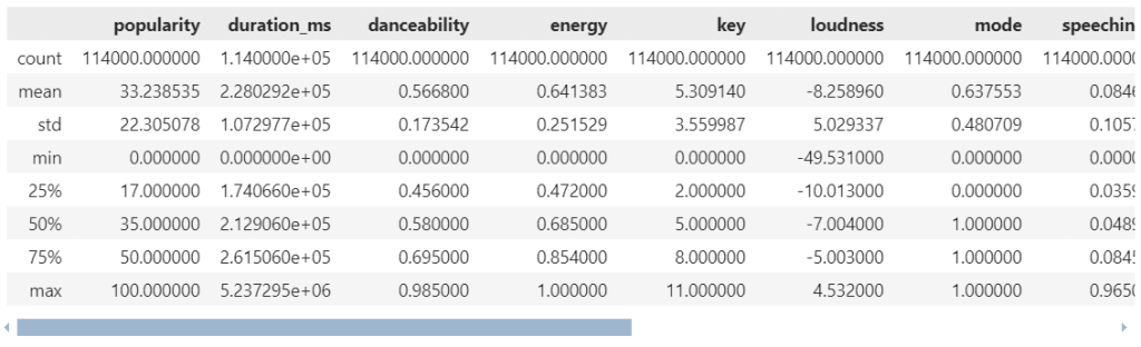
Note:
โดย default, .describe() จะสรุปข้อมูลเฉพาะ column ที่เป็น numerical variable เท่านั้น
ถ้าเราต้องการ summary stats ของ categorical variable เราสามารถใช้ argument include="all" ได้:
# Get summary stats for all variable types
spotify.describe(include="all")
ผลลัพธ์:
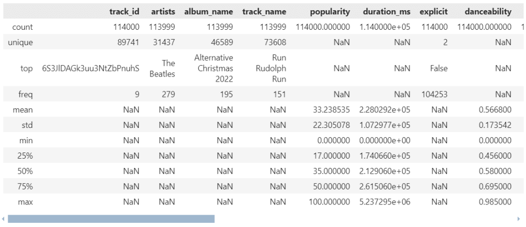
จะเห็นได้ว่า ตอนนี้เราจะได้ summary stats ของทั้ง numerical (เช่น popularity) และ categorical variables (เช่น artists)
.
4️⃣ .shape
Use case:
ดูจำนวน rows และ columns ของ dataset
ตัวอย่าง:
# See the dimensions of the dataset
spotify.shape
ผลลัพธ์:
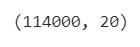
114000คือ จำนวน rows20คือ จำนวน columns
🎶 Playlist #2 – Selecting & Filtering

ในกลุ่มการใช้งานที่ 2 เรามาดูวิธีการเลือกและกรองข้อมูลกัน:
df[condition].query()
.
1️⃣ df[condition]
Use case:
df[condition] เป็น syntax เพื่อกรองข้อมูล
ตัวอย่าง:
เราต้องการดูข้อมูลเพลงที่มีคะแนนความนิยม (popularity) สูงกว่า 80:
# Select records where popularity is greater than 80
spotify[spotify["popularity"] > 80]
ผลลัพธ์:
Note:
ในการกรอง เราสามารถใช้ comparison operators เหล่านี้ช่วยได้:
| Comparison Operator | Meaning |
|---|---|
== | เท่ากับ |
!= | ไม่เท่ากับ |
> | มากกว่า |
>= | มากกว่า/เท่ากับ |
< | น้อยกว่า |
<= | น้อยกว่า/เท่ากับ |
นอกจากนี้ เราสามารถใช้ Boolean operators เพื่อเพิ่ม conditions ในการกรองข้อมูลได้:
| Boolean Operator | Meaning |
|---|---|
& | and |
| ` | ` |
! | not |
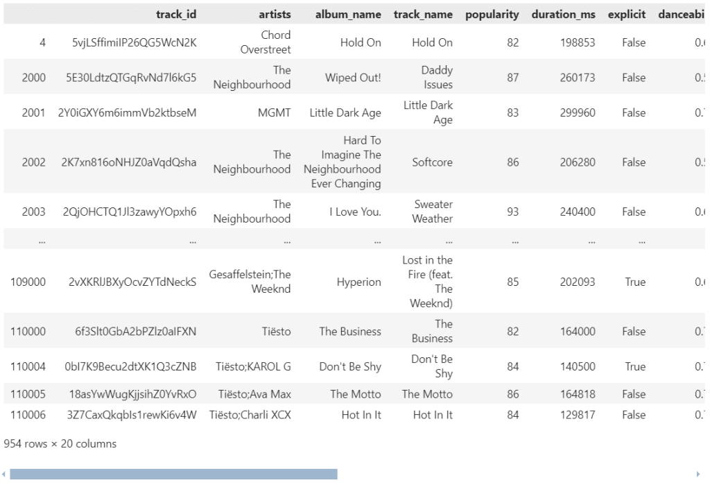
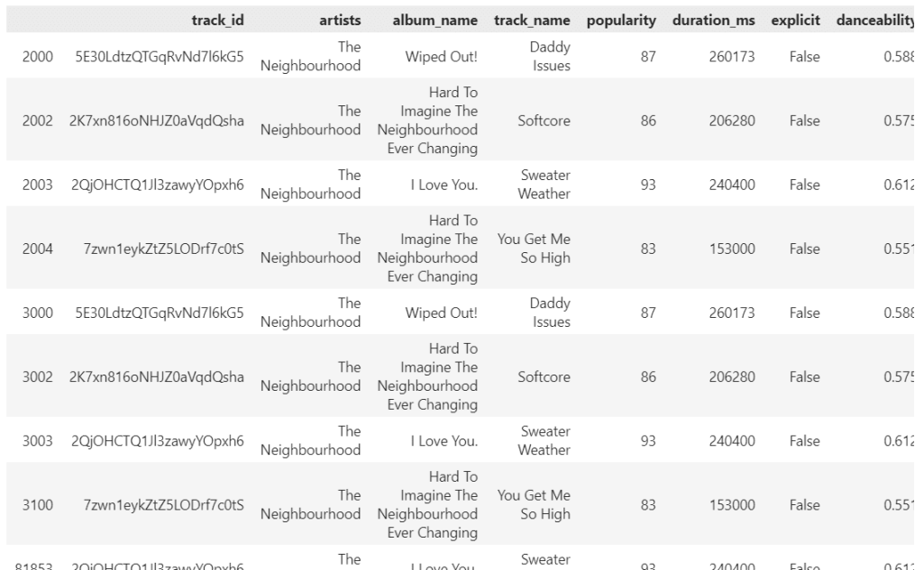
เช่น ดูข้อมูลเพลงที่มีคะแนนความนิยม (popularity) สูงกว่า 80 จากวง The Neighbourhood (ดูจาก artists):
# Select records where popularity is greater than 80 from The Neighbourhood
spotify[(spotify["popularity"] > 80) & (spotify["artists"] == "The Neighbourhood")]
ผลลัพธ์:
.
2️⃣ .query()
Use case:
.query() ทำหน้าที่คล้ายกับ df[condition] นั่นคือ กรองข้อมูล
แต่ .query() มีข้อดีอยู่ 2 อย่าง:
- ใช้งานง่าย
- เหมาะกับการกรองข้อมูล ด้วย conditions ที่ซับซ้อน
การเขียน input ของ .query() เราจะใช้ใน syntax ของ SQL
ตัวอย่าง:
จากตัวอย่างก่อนหน้านี้ที่เราต้องการดูข้อมูลเพลงที่:
- มีคะแนนความนิยม (
popularity) สูงกว่า 80 - จากวง The Neighbourhood (ดูจาก
artists)
เราสามารถเขียน .query() ได้ดังนี้:
# Filter with .query()
spotify.query("popularity > 80 and artists == 'The Neighbourhood'")
ผลลัพธ์:

Note:
ถ้าเราเทียบระหว่าง df[condition] และ .query() :
| df[condition] | .query() |
|---|---|
spotify[(spotify["popularity"] > 80) & (spotify["artists"] == "The Neighbourhood")] | spotify.query("popularity > 80 and artists == 'The Neighbourhood'") |
จะเห็นว่า .query():
- สั้นกว่า
- ทำความเข้าใจได้ง่ายกว่า
🎶 Playlist #3 – Sorting

หลังจากกรองข้อมูล บางครั้งเราอยากจะจัดลำดับข้อมูล เพื่อช่วยในการทำความเข้าใจข้อมูล:
.sort_values()
.
1️⃣ .sort_values()
Use case:
จัดเรียงข้อมูล โดย:
- default จะเรียงจากน้อยไปมาก (A-Z)
- ถ้าต้องการเรียงจากมากไปน้อย (Z-A) ให้ใช้
ascending=False
ตัวอย่าง:
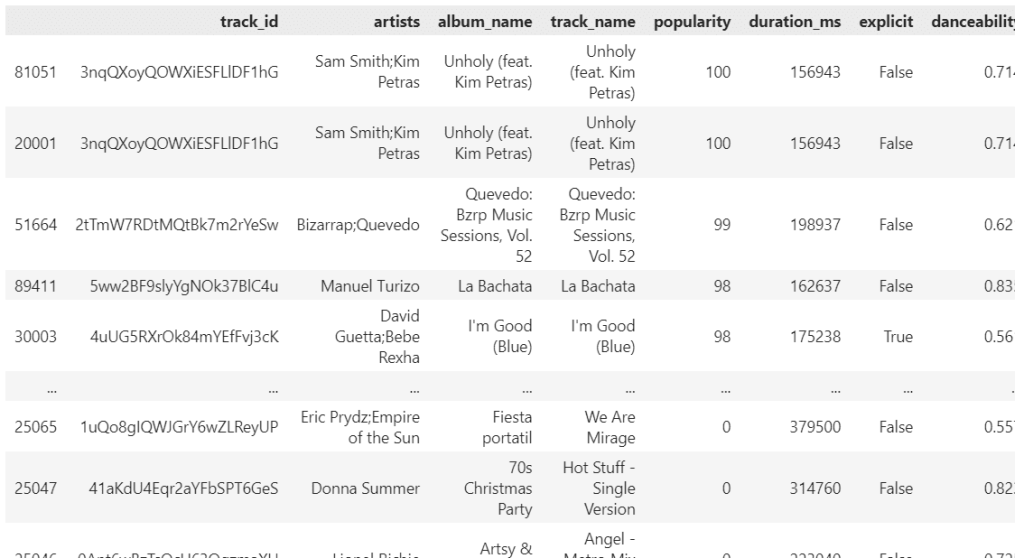
ต้องการเรียงเพลงตามคะแนนความนิยม (popularity) จากสูงไปต่ำ เพื่อหาเพลงฮิต:
# Sort tracks by popularity in descending order
spotify.sort_values(by="popularity", ascending=False)
ผลลัพธ์:
🎶 Playlist #4 – Slicing

ในกลุ่มนี้ เราจะมาดู 4 วิธี เพื่อดึง rows และ/หรือ columns ออกจาก dataset กัน:
df[column].loc[].iloc[].filter()
.
1️⃣ df[column_name]
Use case:
df[column_name] เป็น syntax เพื่อเลือกข้อมูลจาก column ที่ต้องการ โดย:
- df หมายถึง ชื่อ dataset
- column_name หมายถึง ชื่อ column ที่เราเลือก
ตัวอย่าง:
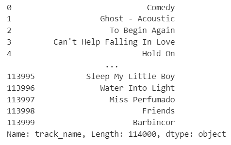
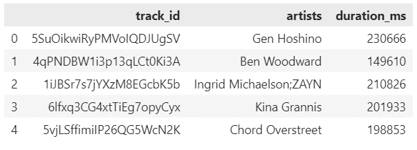
เลือกดูชื่อเพลง (track_name):
# Select column track_name
spotify["track_name"]
ผลลัพธ์:
Note:
ถ้าต้องการมากกว่า 1 column เราสามารถใส่ input เป็น list ได้
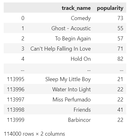
เช่น เลือกชื่อเพลง (track_name) และคะแนนความนิยม (popularity):
# Select columns track_name and popularity
spotify[["track_name", "popularity"]]
ผลลัพธ์:
.
2️⃣ .loc[]
Use case:
เลือก rows และ/หรือ columns โดยใช้ ชื่อ rows และ columns (label-based)
Syntax:
.loc[] มีหลักการใช้งานดังนี้:
| Syntax | For |
|---|---|
df.loc[r_lab] | เลือก 1 row |
df.loc[rx:ry] | เลือกมากกว่า 1 rows |
df.loc[[r_list]] | เลือกมากกว่า 1 rows |
df.loc[:, c_lab] | เลือก 1 column |
df.loc[:, cx:cy] | เลือกมากกว่า 1 column |
df.loc[:, [c_list]] | เลือกมากกว่า 1 columns |
- r_lab คือ ชื่อ row
- rx:ry คือ ช่วง rows ที่ต้องการเลือก
- [r_list] คือ list ของ rows ที่ต้องการเลือก
- c_lab คือ ชื่อ column ที่ต้องการเลือก
- cx:cy คือ ช่วง columns ที่ต้องการเลือก
- [c_list] คือ list ของ columns ที่ต้องการเลือก
ตัวอย่าง:
เลือก 5 rows แรก และแสดงเฉพาะ:
- ชื่อเพลง (
track_name) - ชื่อศิลปิน (
artists) - คะแนนความนิยม (
popularity)
# Select first 5 rows from track_name, artists, popularity
spotify.loc[0:4, ["track_name", "artists", "popularity"]]
ผลลัพธ์:

.
3️⃣ .iloc[]
Use case:
เลือก rows และ/หรือ columns โดยใช้ ตำแหน่ง rows และ columns (position-based)
Syntax:
.iloc[] มีวิธีการใช้งาน คล้ายกับ .loc[] ดังนี้:
| Syntax | For |
|---|---|
df.iloc[r_index] | เลือก 1 row |
df.iloc[rx:ry] | เลือกมากกว่า 1 rows |
df.iloc[[r_list]] | เลือกมากกว่า 1 rows |
df.iloc[:, c_index] | เลือก 1 column |
df.iloc[:, cx:cy] | เลือกมากกว่า 1 column |
df.iloc[:, [c_list]] | เลือกมากกว่า 1 columns |
- r_index คือ ตำแหน่ง row
- rx:ry คือ ช่วง rows ที่ต้องการเลือก
- [r_list] คือ list ของ rows ที่ต้องการเลือก
- c_index คือ ตำแหน่ง column ที่ต้องการเลือก
- cx:cy คือ ช่วง columns ที่ต้องการเลือก
- [c_list] คือ list ของ columns ที่ต้องการเลือก
ความแตกต่างระหว่าง .loc[] และ .iloc[] คือ สิ่งที่ใช้ในการเลือก s และ columns:
.loc[]ใช้ ชื่อ (label).iloc[]ใช้ ตำแหน่ง (position)
ตัวอย่าง:
เลือก 5 rows แรก และแสดงเฉพาะ:
- ชื่อเพลง (
track_name) - ชื่อศิลปิน (
artist_name) - คะแนนความนิยม (
popularity)
# Select first 5 rows from track_name, artists, popularity
spotify.iloc[0:5, [0, 1, 5]]
ผลลัพธ์:
.
4️⃣ .filter()
Use case:
.filter() ทำหน้าที่คล้ายกับ df[condition] แต่ทรงพลังกว่า เพราะเลือกกรองข้อมูลได้ทั้ง rows และ columns
Syntax:
df.filter(condition, axis)
dfคือ ชื่อ datasetconditionคือ เงื่อนไขในการเลือกข้อมูล ซึ่งเรามี 3 parametres ให้เลือกใช้:itemsกรองตาม labels ของ rows หรือ columnslikeกรองตาม คำค้นหาregกรองตาม regular expression
axisระบุว่า ต้องการเลือก rows (0) หรือ columns (1)
ตัวอย่าง:
เลือก rows ที่เลข 123:
# Select rows with "123"
spotify.filter(like="123", axis=0)
ผลลัพธ์:

หรือ เลือกข้อมูลจาก columns:
- ชื่อเพลง (
track_name) - ชื่อศิลปิน (
artist_name) - คะแนนความนิยม (
popularity)
# Select first 5 rows from track_name, artists, popularity
spotify.filter(items=["track_name", "artists", "popularity"])
ผลลัพธ์:

🎶 Playlist #5 – Aggregating

สุดท้าย เรามาดูวิธีการสรุปข้อมูลกัน:
- Aggregation functions
.agg().groupby()
.
1️⃣ Aggregation Functions
ในกรณีที่เราต้องการ คำนวณค่าทางสถิติ pandas มี functions ให้เลือกใช้งานมากมาย เช่น:
| Function | Meaning |
|---|---|
.sum() | หาผลรวม |
.mean() | หาค่าเฉลี่ย |
.median() | หาค่ากลาง |
.mode() | หาค่าที่ซ้ำมากที่สุด |
.min() | หาค่าน้อยที่สุด |
.max() | หาค่ามากที่สุด |
.std() | หา standard deviation (SD) |
.cumsum() | หาผลรวมสะสม |
.value_counts() | นับจำนวนข้อมูล |
.nunique() | นับจำนวนข้อมูลที่ไม่ซ้ำ |
ตัวอย่าง:
ต้องการหาค่าเฉลี่ยของคะแนนความนิยม (popularity):
# Calculate the mean of popularity
spotify["popularity"].mean()
ผลลัพธ์:

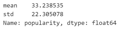
หรือหา SD ของคะแนนความนิยม (popularity):
# Calculate the SD of popularity
spotify["popularity"].std()
ผลลัพธ์:

.
2️⃣ .agg()
Use case:
ในบางครั้ง เราต้องการคำนวณหลายค่าทางสถิติพร้อมกัน เช่น ตัวอย่างก่อนหน้านี้ที่เราต้องการหา mean และ SD
แทนที่เราจะเขียน code เพื่อแสดงผลแยกกัน เช่น:
# Calculate mean
spotify["popularity"].mean()

# Calculate SD
spotify["popularity"].std()
เราสามารถใช้ agg() เพื่อช่วยลดเวลาได้
ตัวอย่าง:
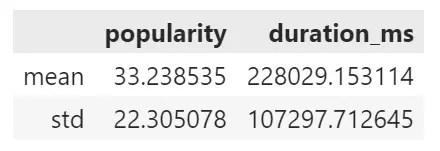
หาค่าเฉลี่ยและ SD ของคะแนนความนิยม (popularity):
# Calculate mean and SD of popularity
spotify["popularity"].agg(["mean", "std"])
ผลลัพธ์:
Note:
เราสามารถใช้ .agg() เพื่อคำนวณค่าทางสถิติกับหลาย column พร้อมกันได้ เช่น หาค่า:
- mean
- std
ให้กับ:
- คะแนนความนิยม
- ความยาวของเพลง
# Calculate mean and SD for popularity and duration_ms
spotify[["popularity", "duration_ms"]].agg({
		"popularity": ["mean", "std"],
		"duration_ms": ["mean", "std"]
		})
ผลลัพธ์:
.
3️⃣ .groupby()
Use case:
บางครั้ง เราต้องการคำนวณค่าทางสถิติตามกลุ่มข้อมูล
เราสามารถใช้ .groupby() เพื่อจับกลุ่มข้อมูล ก่อนจะคำนวณค่าทางสถิติได้
ตัวอย่าง:
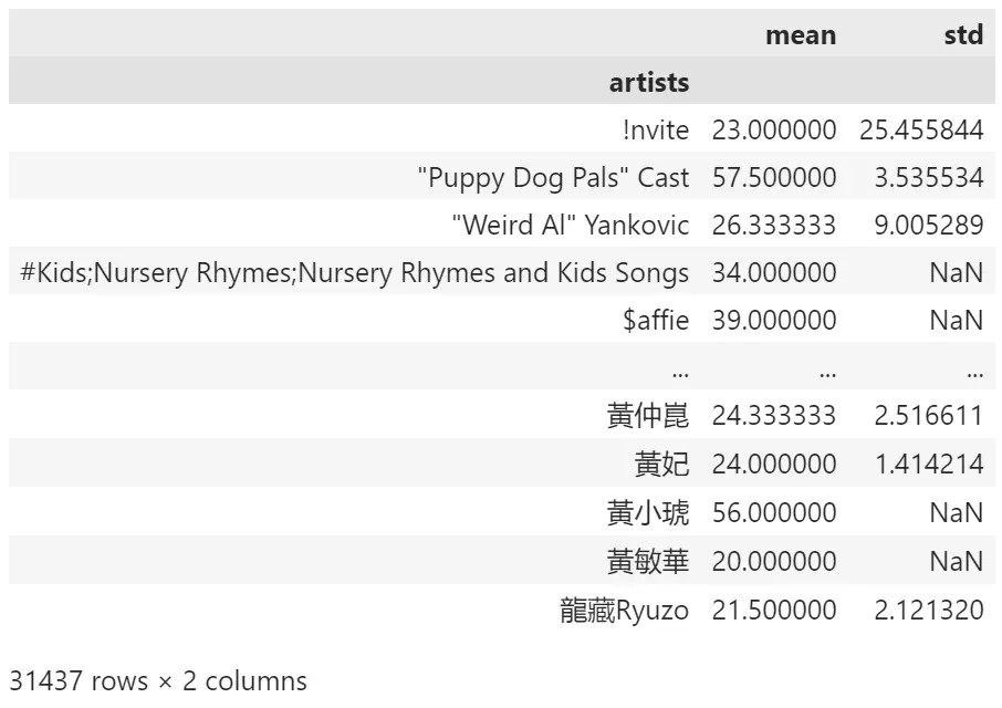
ต้องการหา ค่าเฉลี่ยและ SD ของคะแนนความนิยม (popularity) ของศิลปินแต่ละคน:
# Group by artists and calculate mean of popularity
spotify.groupby("artists")["popularity"].agg(["mean", "std"])
ผลลัพธ์:
⏭️ Next Song
.
💻 Example Code
สำหรับคนที่ลองรัน code ด้วยตัวเอง สามารถโหลด code ตัวอย่างได้ที่ GitHub
.
📚 Further Reading
สำหรับคนที่สนใจเรียนรู้เพิ่มเติมเกี่ยวกับ pandas สามารถศึกษาต่อได้ตาม links ด้านล่าง:
