Category: R

Basic R—รวบรวม 13 บทความสอนทำงานกับ data ในภาษา R: Intro to R, Importing Data, Data Manipulation, และ Data Visualisation
ในปีนี้ ผมเริ่มหันมาฝึกใช้ภาษา R อย่างจริงจังมากขึ้น หลังจากเรียนคอร์สออนไลน์จาก DataRockie และ DataCamp มา

และเพื่อช่วยให้ผมเข้าใจภาษา R มากขึ้น ผมได้เขียนสรุปการใช้งานภาษา R เบื้องต้นไว้ ทั้งหมด 13 บทความ ซึ่งผมได้รวบรวมไว้เป็น 4 กลุ่ม ดังนี้:
1. Introduction to R: แนะนำภาษา R และการทำงานกับ R เบื้องต้น
2. Importing data: การนำเข้าข้อมูลในภาษา R
3. Data manipulation: การแปลงข้อมูลดิบให้พร้อมสำหรับการวิเคราะห์
4. Data visualisation: การแสดงข้อมูลในรูปแบบกราฟ
.

Group 1. Introduction to R (3 บทความ):
1. R foundation: แนะนำภาษา R—ความแตกต่างระหว่าง R และ Python, data types, และ data structures ในภาษา R
2. R control flow: สอนใช้ if, for, while เพื่อควบคุมการทำงานของภาษา R
3. R functions (รอลงบทความนะครับ 😆): สอนสร้างและใช้งาน functions ในภาษา R
.

Group 2. Importing data (5 บทความ):
1. Working with data frame: แนะนำ 10 วิธีในการทำงานกับ data frame ซึ่งเป็น data structure ที่พบบ่อยที่สุดในภาษา R
2. Working with data frame using SQL: สอนการทำงานกับ data frame ด้วย SQL
3. Working with flat files (รอลงบทความนะครับ 😆): แนะนำการใช้ 3 packages สำหรับ import ข้อมูลจาก flat files
4. Working with Excel: แนะนำ 2 packages สำหรับทำงานกับ Excel
5. Working with database: แนะนำวิธีทำงานกับ database ผ่าน DBI package
.

Group 3. Data manipulation (4 บทความ):
1. dplyr package: แนะนำ 5 functions ยอดนิยมสำหรับ data manipulation
2. dbplyr package: แนะนำการใช้ dplyr functions เพื่อทำงานกับ database
3. dtplyr package: แนะนำการใช้ dplyr functions เพื่อทำงานกับข้อมูลขนาดใหญ่
4. data.table package: แนะนำ package ยอดนิยมสำหรับทำงานกับข้อมูลขนาดใหญ่
.

Group 4. Data visualisation (1 บทความ):
1. ggplot2 package: แนะนำวิธีใช้ package เพื่อสร้าง data viz แบบองค์กรระดับโลก
👉 Tie-In: Machine Learning in R

สำหรับคนที่สนใจ machine learning ในภาษา R สามารถดู 13 บทความการทำ machine learning ในรูปแบบต่าง ๆ ได้ที่นี่

✅ R Book for Psychologists: หนังสือภาษา R สำหรับนักจิตวิทยา

📕 ขอฝากหนังสือเล่มแรกในชีวิตด้วยนะครับ 😆

🙋 ใครที่กำลังเรียนจิตวิทยาหรือทำงานสายจิตวิทยา และเบื่อที่ต้องใช้ software ราคาแพงอย่าง SPSS และ Excel เพื่อทำข้อมูล

💪 ผมขอแนะนำ R Book for Psychologists หนังสือสอนใช้ภาษา R เพื่อการวิเคราะห์ข้อมูลทางจิตวิทยา ที่เขียนมาเพื่อนักจิตวิทยาที่ไม่เคยมีประสบการณ์เขียน code มาก่อน

ในหนังสือ เราจะปูพื้นฐานภาษา R และพาไปดูวิธีวิเคราะห์สถิติที่ใช้บ่อยกัน เช่น:
- Correlation
- t-tests
- ANOVA
- Reliability
- Factor analysis
🚀 เมื่ออ่านและทำตามตัวอย่างใน R Book for Psychologists ทุกคนจะไม่ต้องพึง SPSS และ Excel ในการทำงานอีกต่อไป และสามารถวิเคราะห์ข้อมูลด้วยตัวเองได้ด้วยความมั่นใจ

แล้วทุกคนจะแปลกใจว่า ทำไมภาษา R ง่ายขนาดนี้ 🙂‍↕️

👉 สนใจดูรายละเอียดหนังสือได้ที่ meb:

ดูรายละเอียดหนังสือ R Book for Psychologists
Share this:
X
Facebook
Like Loading…
2025-12-30

สรุป 10 วิธีในการทำงานกับ data frame ในภาษา R: creating, indexing, subsetting, filtering, sorting, และอื่น ๆ — ตัวอย่างการทำงานกับ Jujutsu Kaisen data frame

Data frame เป็นหนึ่งใน data structure ที่พบบ่อยที่สุดในการทำงานกับข้อมูล

Data frame เก็บข้อมูลในรูปแบบตาราง โดย:

1 row = 1 รายการ (เช่น ข้อมูลของ John)
1 column = 1 ประเภทข้อมูล (เช่น อายุ)

ตัวอย่าง data frame:

ในบทความนี้ เราจะมาสรุป 10 วิธีในการทำงานกับ data frame กัน:

Creating: การสร้าง data frame
Previewing: การดูข้อมูล data frame
Indexing: การเลือก columns ที่ต้องการ
Subsetting: การเลือก rows และ columns ที่ต้องการ
Filtering: การกรองข้อมูล
Sorting: การจัดลำดับข้อมูล
Aggregating: การสรุปข้อมูล
Adding columns: การเพิ่ม columns ใหม่
Removing columns: การลบ columns
Binding: การเชื่อมข้อมูลใหม่เข้ากับ data frame

ถ้าพร้อมแล้ว ไปเริ่มกันเลย

1️⃣ Creating

เราสามารถสร้าง data frame ด้วย data.frame() ซึ่งต้องการ ชื่อ column และ vector ที่เก็บข้อมูลของ column นั้น ๆ:

# Create a data frame
jjk_df <- data.frame(
  ID = 1:10,
  Name = c("Yuji Itadori", "Megumi Fushiguro", "Nobara Kugisaki", "Satoru Gojo",
           "Maki Zenin", "Toge Inumaki", "Panda", "Kento Nanami", "Yuta Okkotsu", "Suguru Geto"),
  Age = c(15, 16, 16, 28, 17, 17, 18, 27, 17, 27),
  Grade = c("1st Year", "1st Year", "1st Year", "Special", "2nd Year",
            "2nd Year", "2nd Year", "Special", "Special", "Special"),
  CursedEnergy = c(80, 95, 70, 999, 60, 85, 75, 200, 300, 400),
  Technique = c("Divergent Fist", "Ten Shadows", "Straw Doll", "Limitless",
                "Heavenly Restriction", "Cursed Speech", "Gorilla Mode",
                "Ratio Technique", "Rika", "Cursed Spirit Manipulation"),
  Missions = c(25, 30, 20, 120, 35, 28, 40, 90, 55, 80)
)

# View the result
jjk_df

ผลลัพธ์:

   ID             Name Age    Grade CursedEnergy                  Technique Missions
1   1     Yuji Itadori  15 1st Year           80             Divergent Fist       25
2   2 Megumi Fushiguro  16 1st Year           95                Ten Shadows       30
3   3  Nobara Kugisaki  16 1st Year           70                 Straw Doll       20
4   4      Satoru Gojo  28  Special          999                  Limitless      120
5   5       Maki Zenin  17 2nd Year           60       Heavenly Restriction       35
6   6     Toge Inumaki  17 2nd Year           85              Cursed Speech       28
7   7            Panda  18 2nd Year           75               Gorilla Mode       40
8   8     Kento Nanami  27  Special          200            Ratio Technique       90
9   9     Yuta Okkotsu  17  Special          300                       Rika       55
10 10      Suguru Geto  27  Special          400 Cursed Spirit Manipulation       80

2️⃣ Previewing

เรามี 8 functions สำหรับดูข้อมูล data frame:

No.	Function	For
1	`View()`	ดูข้อมูลทั้งหมด
2	`head()`	ดูข้อมูล 6 rows แรก
3	`tail()`	ดูข้อมูล 6 rows สุดท้าย
4	`str()`	ดูโครงสร้างข้อมูล
5	`summary()`	ดูสถิติข้อมูล
6	`dim()`	ดูจำนวน rows และ columns
7	`nrow()`	ดูจำนวน rows
8	`ncol()`	ดูจำนวน columns

เราไปดูตัวอย่างทั้ง 8 functions กัน

👀 View()

View() ใช้ดูข้อมูลทั้งหมดใน data frame:

# View the whole data frame
View(jjk_df)

เราจะเห็นผลลัพธ์ในหน้าต่างใหม่:

Note: เนื่องจาก View() แสดงข้อมูลทั้งหมด จึงเหมาะกับการใช้งานกับ data frame ขนาดเล็ก

🙊 head()

head() ใช้ดูข้อมูล 6 rows แรกใน data frame:

# View the first 6 rows
head(jjk_df)

ผลลัพธ์:

  ID             Name Age    Grade CursedEnergy            Technique Missions
1  1     Yuji Itadori  15 1st Year           80       Divergent Fist       25
2  2 Megumi Fushiguro  16 1st Year           95          Ten Shadows       30
3  3  Nobara Kugisaki  16 1st Year           70           Straw Doll       20
4  4      Satoru Gojo  28  Special          999            Limitless      120
5  5       Maki Zenin  17 2nd Year           60 Heavenly Restriction       35
6  6     Toge Inumaki  17 2nd Year           85        Cursed Speech       28

🐒 tail()

tail() ใช้ดูข้อมูล 6 rows สุดท้ายใน data frame:

# View the last 6 rows
tail(jjk_df)

ผลลัพธ์:

   ID         Name Age    Grade CursedEnergy                  Technique Missions
5   5   Maki Zenin  17 2nd Year           60       Heavenly Restriction       35
6   6 Toge Inumaki  17 2nd Year           85              Cursed Speech       28
7   7        Panda  18 2nd Year           75               Gorilla Mode       40
8   8 Kento Nanami  27  Special          200            Ratio Technique       90
9   9 Yuta Okkotsu  17  Special          300                       Rika       55
10 10  Suguru Geto  27  Special          400 Cursed Spirit Manipulation       80

🏗️ str()

str() ใช้ดูโครงสร้างข้อมูลของ data frame:

# View the data frame structure
str(jjk_df)

ผลลัพธ์:

'data.frame':	10 obs. of  7 variables:
 $ ID          : int  1 2 3 4 5 6 7 8 9 10
 $ Name        : chr  "Yuji Itadori" "Megumi Fushiguro" "Nobara Kugisaki" "Satoru Gojo" ...
 $ Age         : num  15 16 16 28 17 17 18 27 17 27
 $ Grade       : chr  "1st Year" "1st Year" "1st Year" "Special" ...
 $ CursedEnergy: num  80 95 70 999 60 85 75 200 300 400
 $ Technique   : chr  "Divergent Fist" "Ten Shadows" "Straw Doll" "Limitless" ...
 $ Missions    : num  25 30 20 120 35 28 40 90 55 80

จากผลลัพธ์ เราจะเห็นข้อมูล 5 อย่าง ได้แก่:

จำนวน rows (obs.)
จำนวน columns (variables)
ชื่อ columns (เช่น ID)
ประเภทข้อมูลของแต่ละ column (เช่น int)
ตัวอย่างข้อมูลของแต่ละ column (เช่น 1 2 3 4 5 6 7 8 9 10)

🧮 summary()

summary() ใช้สรุปข้อมูลใน data frame เช่น:

ค่าเฉลี่ย (Mean)
จำนวนข้อมูล (Length)

# View the summary
summary(jjk_df)

ผลลัพธ์:

       ID            Name                Age           Grade            CursedEnergy     Technique            Missions     
 Min.   : 1.00   Length:10          Min.   :15.00   Length:10          Min.   : 60.00   Length:10          Min.   : 20.00  
 1st Qu.: 3.25   Class :character   1st Qu.:16.25   Class :character   1st Qu.: 76.25   Class :character   1st Qu.: 28.50  
 Median : 5.50   Mode  :character   Median :17.00   Mode  :character   Median : 90.00   Mode  :character   Median : 37.50  
 Mean   : 5.50                      Mean   :19.80                      Mean   :236.40                      Mean   : 52.30  
 3rd Qu.: 7.75                      3rd Qu.:24.75                      3rd Qu.:275.00                      3rd Qu.: 73.75  
 Max.   :10.00                      Max.   :28.00                      Max.   :999.00                      Max.   :120.00

💠 dim()

dim() ใช้แสดงจำนวน rows และ columns ใน data frame:

# View the dimensions
dim(jjk_df)

ผลลัพธ์:

[1] 10  7

🚣 nrow()

nrow() ใช้แสดงจำนวน rows ใน data frame:

# Get the number of rows
nrow(jjk_df)

ผลลัพธ์:

[1] 10

🏦 ncol()

ncol() ใช้แสดงจำนวน columns ใน data frame:

# Get the number of columns
ncol(jjk_df)

ผลลัพธ์:

[1] 7

3️⃣ Indexing

Indexing หมายถึง การเลือก columns ที่ต้องการ ซึ่งเราทำได้ 2 วิธี:

ใช้ $ (นิยมใช้)
ใช้ [[]]

💰 Using $

เราสามารถใช้ $ ได้แบบนี้:

df$col

ยกตัวอย่างเช่น เลือก column Name:

# Index with $
jjk_df$Name

ผลลัพธ์:

 [1] "Yuji Itadori"     "Megumi Fushiguro" "Nobara Kugisaki"  "Satoru Gojo"      "Maki Zenin"      
 [6] "Toge Inumaki"     "Panda"            "Kento Nanami"     "Yuta Okkotsu"     "Suguru Geto"

🔳 Using [[]]

เราสามารถใช้ [[]] ได้แบบนี้:

df[["col"]]

ยกตัวอย่างเช่น เลือก column Name:

# Index with [[]]
jjk_df[["Name"]]

ผลลัพธ์:

 [1] "Yuji Itadori"     "Megumi Fushiguro" "Nobara Kugisaki"  "Satoru Gojo"      "Maki Zenin"      
 [6] "Toge Inumaki"     "Panda"            "Kento Nanami"     "Yuta Okkotsu"     "Suguru Geto"

4️⃣ Subsetting

Subsetting คือ การเลือก rows และ columns จาก data frame ซึ่งเราทำได้ 2 วิธี:

ใช้ df[rows, cols] syntax
ใช้ subset()

🍽️ df[rows, cols]

เราสามารถใช้ df[rows, cols] ได้ 3 แบบ:

เลือก rows
เลือก columns
เลือก rows และ columns

แบบที่ 1. เลือก rows อย่างเดียว:

# Subset rows only
jjk_df[1:5, ]

ผลลัพธ์:

  ID             Name Age    Grade CursedEnergy            Technique Missions
1  1     Yuji Itadori  15 1st Year           80       Divergent Fist       25
2  2 Megumi Fushiguro  16 1st Year           95          Ten Shadows       30
3  3  Nobara Kugisaki  16 1st Year           70           Straw Doll       20
4  4      Satoru Gojo  28  Special          999            Limitless      120
5  5       Maki Zenin  17 2nd Year           60 Heavenly Restriction       35

แบบที่ 2. เลือก columns อย่างเดียว:

# Subset columns only
jjk_df[, "Name"]

ผลลัพธ์:

 [1] "Yuji Itadori"     "Megumi Fushiguro" "Nobara Kugisaki"  "Satoru Gojo"      "Maki Zenin"      
 [6] "Toge Inumaki"     "Panda"            "Kento Nanami"     "Yuta Okkotsu"     "Suguru Geto"

แบบที่ 3. เลือก rows และ columns:

# Subset rows and columns
jjk_df[1:5, c("Name", "Technique")]

ผลลัพธ์:

              Name            Technique
1     Yuji Itadori       Divergent Fist
2 Megumi Fushiguro          Ten Shadows
3  Nobara Kugisaki           Straw Doll
4      Satoru Gojo            Limitless
5       Maki Zenin Heavenly Restriction

🔪 subset()

เราสามารถ subset ข้อมูลได้ด้วย subset() ซึ่งต้องการ 2 arguments:

subset(x, select)

x = data frame
select = columns ที่ต้องการเลือก

# Subset using susbet() - select conlumns only
subset(jjk_df, select = c("Name", "Technique"))

ผลลัพธ์:

               Name                  Technique
1      Yuji Itadori             Divergent Fist
2  Megumi Fushiguro                Ten Shadows
3   Nobara Kugisaki                 Straw Doll
4       Satoru Gojo                  Limitless
5        Maki Zenin       Heavenly Restriction
6      Toge Inumaki              Cursed Speech
7             Panda               Gorilla Mode
8      Kento Nanami            Ratio Technique
9      Yuta Okkotsu                       Rika
10      Suguru Geto Cursed Spirit Manipulation

ในกรณีที่เราต้องการเลือก rows ด้วย เราจะต้องกำหนด rows ใน x:

# Subset using susbet() - select both rows and columns
subset(jjk_df[1:5, ], select = c("Name", "Technique"))

ผลลัพธ์:

              Name            Technique
1     Yuji Itadori       Divergent Fist
2 Megumi Fushiguro          Ten Shadows
3  Nobara Kugisaki           Straw Doll
4      Satoru Gojo            Limitless
5       Maki Zenin Heavenly Restriction

5️⃣ Filtering

เราสามารถกรองข้อมูลใน data frame ได้ 2 วิธี:

ใช้ df[rows, cols] syntax
ใช้ subset()

🍽️ df[rows, cols]

เราสามารถกรองข้อมูลด้วย df[rows, cols] โดยกำหนดเงื่อนไขการกรองใน rows

เช่น กรองข้อมูลตัวละครที่อยู่ปี 1:

# Filter using df[rows, cols] - 1 condition
jjk_df[jjk_df$Grade == "1st Year", ]

ผลลัพธ์:

  ID             Name Age    Grade CursedEnergy      Technique Missions
1  1     Yuji Itadori  15 1st Year           80 Divergent Fist       25
2  2 Megumi Fushiguro  16 1st Year           95    Ten Shadows       30
3  3  Nobara Kugisaki  16 1st Year           70     Straw Doll       20

ในกรณีที่เรามีมากกว่า 1 เงื่อนไข เราสามารถใช้ logical operators ช่วยได้:

Operator	Meaning
`&`	AND
`\|`	OR
`!`	NOT

ยกตัวอย่างเช่น กรองข้อมูลตัวละครที่อยู่ปี 1 และมีอายุ 15 ปี:

# Filter using df[rows, cols] - multiple conditions
jjk_df[jjk_df$Grade == "1st Year" & jjk_df$Age == 15, ]

ผลลัพธ์:

  ID         Name Age    Grade CursedEnergy      Technique Missions
1  1 Yuji Itadori  15 1st Year           80 Divergent Fist       25

🔪 subset()

เราสามารถใช้ subset() เพื่อกรองข้อมูลได้แบบนี้:

# Filter using subset() - 1 condition
subset(jjk_df, Grade == "1st Year")

ผลลัพธ์:

  ID             Name Age    Grade CursedEnergy      Technique Missions
1  1     Yuji Itadori  15 1st Year           80 Divergent Fist       25
2  2 Megumi Fushiguro  16 1st Year           95    Ten Shadows       30
3  3  Nobara Kugisaki  16 1st Year           70     Straw Doll       20

เราสามารถเพิ่มเงื่อนไขการกรองได้ด้วย logical operator เช่น:

# Filter using subset() - multiple conditions
subset(jjk_df, Grade == "1st Year" & Age == 15)

ผลลัพธ์:

  ID         Name Age    Grade CursedEnergy      Technique Missions
1  1 Yuji Itadori  15 1st Year           80 Divergent Fist       25

6️⃣ Sorting

สำหรับการเรียงข้อมูล เราจะใช้ order() ซึ่งเพื่อเรียงข้อมูลได้ 3 แบบ:

Ascending (A–Z)
Descending (Z–A)
Sort by multiple columns: จัดเรียงด้วยหลาย columns

⬇️ Ascending

ยกตัวอย่างเช่น เรียงลำดับตามจำนวนภารกิจ (Missions):

# Sort ascending (default)
jjk_df[order(jjk_df$Missions), ]

ผลลัพธ์:

   ID             Name Age    Grade CursedEnergy                  Technique Missions
3   3  Nobara Kugisaki  16 1st Year           70                 Straw Doll       20
1   1     Yuji Itadori  15 1st Year           80             Divergent Fist       25
6   6     Toge Inumaki  17 2nd Year           85              Cursed Speech       28
2   2 Megumi Fushiguro  16 1st Year           95                Ten Shadows       30
5   5       Maki Zenin  17 2nd Year           60       Heavenly Restriction       35
7   7            Panda  18 2nd Year           75               Gorilla Mode       40
9   9     Yuta Okkotsu  17  Special          300                       Rika       55
10 10      Suguru Geto  27  Special          400 Cursed Spirit Manipulation       80
8   8     Kento Nanami  27  Special          200            Ratio Technique       90
4   4      Satoru Gojo  28  Special          999                  Limitless      120

⬆️ Descending

เราสามารถเรียงข้อมูลแบบ descending ได้ 2 วิธี:

ใช้ decreasing
ใช้ -

วิธีที่ 1. ใช้ decreasing:

# Sort descending with decreasing
jjk_df[order(jjk_df$Missions, decreasing = TRUE), ]

ผลลัพธ์:

   ID             Name Age    Grade CursedEnergy                  Technique Missions
4   4      Satoru Gojo  28  Special          999                  Limitless      120
8   8     Kento Nanami  27  Special          200            Ratio Technique       90
10 10      Suguru Geto  27  Special          400 Cursed Spirit Manipulation       80
9   9     Yuta Okkotsu  17  Special          300                       Rika       55
7   7            Panda  18 2nd Year           75               Gorilla Mode       40
5   5       Maki Zenin  17 2nd Year           60       Heavenly Restriction       35
2   2 Megumi Fushiguro  16 1st Year           95                Ten Shadows       30
6   6     Toge Inumaki  17 2nd Year           85              Cursed Speech       28
1   1     Yuji Itadori  15 1st Year           80             Divergent Fist       25
3   3  Nobara Kugisaki  16 1st Year           70                 Straw Doll       20

วิธีที่ 2. ใช้ -:

# Sort descending with -
jjk_df[order(-jjk_df$Missions), ]

ผลลัพธ์:

   ID             Name Age    Grade CursedEnergy                  Technique Missions
4   4      Satoru Gojo  28  Special          999                  Limitless      120
8   8     Kento Nanami  27  Special          200            Ratio Technique       90
10 10      Suguru Geto  27  Special          400 Cursed Spirit Manipulation       80
9   9     Yuta Okkotsu  17  Special          300                       Rika       55
7   7            Panda  18 2nd Year           75               Gorilla Mode       40
5   5       Maki Zenin  17 2nd Year           60       Heavenly Restriction       35
2   2 Megumi Fushiguro  16 1st Year           95                Ten Shadows       30
6   6     Toge Inumaki  17 2nd Year           85              Cursed Speech       28
1   1     Yuji Itadori  15 1st Year           80             Divergent Fist       25
3   3  Nobara Kugisaki  16 1st Year           70                 Straw Doll       20

↔️ Sort by Multiple Columns

เราสามารถจัดเรียงข้อมูลได้มากกว่า 1 column ด้วยการเลือก columns ที่ต้องการจัดเรียงเพิ่ม

เช่น จัดเรียงด้วย:

Grade
จำนวนภารกิจ (Missions)

# Sort by multiple columns
jjk_df[order(jjk_df$Grade, jjk_df$Missions), ]

ผลลัพธ์:

   ID             Name Age    Grade CursedEnergy                  Technique Missions
3   3  Nobara Kugisaki  16 1st Year           70                 Straw Doll       20
1   1     Yuji Itadori  15 1st Year           80             Divergent Fist       25
2   2 Megumi Fushiguro  16 1st Year           95                Ten Shadows       30
6   6     Toge Inumaki  17 2nd Year           85              Cursed Speech       28
5   5       Maki Zenin  17 2nd Year           60       Heavenly Restriction       35
7   7            Panda  18 2nd Year           75               Gorilla Mode       40
9   9     Yuta Okkotsu  17  Special          300                       Rika       55
10 10      Suguru Geto  27  Special          400 Cursed Spirit Manipulation       80
8   8     Kento Nanami  27  Special          200            Ratio Technique       90
4   4      Satoru Gojo  28  Special          999                  Limitless      120

7️⃣ Aggregating

เราสามารถสรุปข้อมูลโดยใช้ statistics functions เช่น:

Function	For
`mean()`	หาค่าเฉลี่ย
`median()`	หาค่ามัธยฐาน
`min()`	หาค่าต่ำสุด
`max()`	หาค่าสูงสุด
`sd()`	หาค่า standard deviation

ยกตัวอย่างเช่น หาค่าเฉลี่ย Cursed Energy (CursedEnergy):

# Find average Cursed Energy
mean(jjk_df$CursedEnergy)

ผลลัพธ์:

[1] 236.4

8️⃣ Adding Columns

เราสามารถเพิ่ม columns ใหม่ได้ด้วยแบบนี้:

df$new_col <- value

ยกตัวอย่างเช่น เพิ่ม column Ranking:

# Add a column
jjk_df$Ranking <- ifelse(jjk_df$CursedEnergy > 100, "High", "Low")

# View the result
jjk_df

ผลลัพธ์:

   ID             Name Age    Grade CursedEnergy                  Technique Missions Ranking
1   1     Yuji Itadori  15 1st Year           80             Divergent Fist       25     Low
2   2 Megumi Fushiguro  16 1st Year           95                Ten Shadows       30     Low
3   3  Nobara Kugisaki  16 1st Year           70                 Straw Doll       20     Low
4   4      Satoru Gojo  28  Special          999                  Limitless      120    High
5   5       Maki Zenin  17 2nd Year           60       Heavenly Restriction       35     Low
6   6     Toge Inumaki  17 2nd Year           85              Cursed Speech       28     Low
7   7            Panda  18 2nd Year           75               Gorilla Mode       40     Low
8   8     Kento Nanami  27  Special          200            Ratio Technique       90    High
9   9     Yuta Okkotsu  17  Special          300                       Rika       55    High
10 10      Suguru Geto  27  Special          400 Cursed Spirit Manipulation       80    High

9️⃣ Removing Columns

เราสามารถลบ columns ได้ด้วยวิธีเดียวกันกับการเพิ่ม columns:

df$col <- NULL

ยกตัวอย่างเช่น ลบ column Ranking:

# Remove a column
jjk_df$Ranking <- NULL

# View the result
jjk_df

ผลลัพธ์:

   ID             Name Age    Grade CursedEnergy                  Technique Missions
1   1     Yuji Itadori  15 1st Year           80             Divergent Fist       25
2   2 Megumi Fushiguro  16 1st Year           95                Ten Shadows       30
3   3  Nobara Kugisaki  16 1st Year           70                 Straw Doll       20
4   4      Satoru Gojo  28  Special          999                  Limitless      120
5   5       Maki Zenin  17 2nd Year           60       Heavenly Restriction       35
6   6     Toge Inumaki  17 2nd Year           85              Cursed Speech       28
7   7            Panda  18 2nd Year           75               Gorilla Mode       40
8   8     Kento Nanami  27  Special          200            Ratio Technique       90
9   9     Yuta Okkotsu  17  Special          300                       Rika       55
10 10      Suguru Geto  27  Special          400 Cursed Spirit Manipulation       80

🔟 Binding

เราสามารถเชื่อม data frame ได้ 2 แบบ:

rbind(): เชื่อม row
cbind(): เชื่อม column

🤝 rbind()

rbind() ใช้เชื่อม data frame กับ row ใหม่ และต้องการ 2 arguments:

rbind(df1, df2)

df1 = data frame ที่ 1
df2 = data frame ที่ 2

ยกตัวอย่างเช่น เพิ่มชื่อตัวละครใหม่ (Hajime Kashimo):

# Create a new data frame
new_sorcerer <- data.frame(
  ID = 11,
  Name = "Hajime Kashimo",
  Age = 25,
  Grade = "Special",
  CursedEnergy = 500,
  Technique = "Lightning",
  Missions = 60
)

# Bind the data frames by rows
jjk_df <- rbind(jjk_df, new_sorcerer)

# View the result
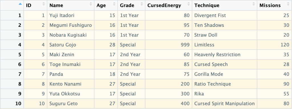
jjk_df

ผลลัพธ์:

   ID             Name Age    Grade CursedEnergy                  Technique Missions
1   1     Yuji Itadori  15 1st Year           80             Divergent Fist       25
2   2 Megumi Fushiguro  16 1st Year           95                Ten Shadows       30
3   3  Nobara Kugisaki  16 1st Year           70                 Straw Doll       20
4   4      Satoru Gojo  28  Special          999                  Limitless      120
5   5       Maki Zenin  17 2nd Year           60       Heavenly Restriction       35
6   6     Toge Inumaki  17 2nd Year           85              Cursed Speech       28
7   7            Panda  18 2nd Year           75               Gorilla Mode       40
8   8     Kento Nanami  27  Special          200            Ratio Technique       90
9   9     Yuta Okkotsu  17  Special          300                       Rika       55
10 10      Suguru Geto  27  Special          400 Cursed Spirit Manipulation       80
11 11   Hajime Kashimo  25  Special          500                  Lightning       60

🤲 cbind()

cbind() ใช้เชื่อม data frame กับ column ใหม่ และต้องการ 2 arguments ได้แก่:

cbind(df, vector)

df = data frame
vector = vector ที่เก็บข้อมูลของ column ใหม่

ยกตัวอย่างเช่น เพิ่ม column ที่บอกว่าตัวละครเป็นครูหรือไม่ (IsTeacher):

# Bind a column
jjk_df <- cbind(
  jjk_df,
  IsTeacher = c(FALSE, FALSE, FALSE, TRUE, FALSE,
                FALSE, FALSE, TRUE, FALSE, TRUE, FALSE)
)

# View the result
jjk_df

ผลลัพธ์:

   ID             Name Age    Grade CursedEnergy                  Technique Missions IsTeacher
1   1     Yuji Itadori  15 1st Year           80             Divergent Fist       25     FALSE
2   2 Megumi Fushiguro  16 1st Year           95                Ten Shadows       30     FALSE
3   3  Nobara Kugisaki  16 1st Year           70                 Straw Doll       20     FALSE
4   4      Satoru Gojo  28  Special          999                  Limitless      120      TRUE
5   5       Maki Zenin  17 2nd Year           60       Heavenly Restriction       35     FALSE
6   6     Toge Inumaki  17 2nd Year           85              Cursed Speech       28     FALSE
7   7            Panda  18 2nd Year           75               Gorilla Mode       40     FALSE
8   8     Kento Nanami  27  Special          200            Ratio Technique       90      TRUE
9   9     Yuta Okkotsu  17  Special          300                       Rika       55     FALSE
10 10      Suguru Geto  27  Special          400 Cursed Spirit Manipulation       80      TRUE
11 11   Hajime Kashimo  25  Special          500                  Lightning       60     FALSE

😺 GitHub

ดูตัวอย่าง code ในบทความนี้ได้ที่ GitHub

📃 References

รูปประกอบจาก Jujutsu Kaisen Character Dataset
R Data Frames
DataFrame Operations in R

✅ R Book for Psychologists: หนังสือภาษา R สำหรับนักจิตวิทยา

📕 ขอฝากหนังสือเล่มแรกในชีวิตด้วยนะครับ 😆

🙋 ใครที่กำลังเรียนจิตวิทยาหรือทำงานสายจิตวิทยา และเบื่อที่ต้องใช้ software ราคาแพงอย่าง SPSS และ Excel เพื่อทำข้อมูล

💪 ผมขอแนะนำ R Book for Psychologists หนังสือสอนใช้ภาษา R เพื่อการวิเคราะห์ข้อมูลทางจิตวิทยา ที่เขียนมาเพื่อนักจิตวิทยาที่ไม่เคยมีประสบการณ์เขียน code มาก่อน

ในหนังสือ เราจะปูพื้นฐานภาษา R และพาไปดูวิธีวิเคราะห์สถิติที่ใช้บ่อยกัน เช่น:

Correlation
t-tests
ANOVA
Reliability
Factor analysis

🚀 เมื่ออ่านและทำตามตัวอย่างใน R Book for Psychologists ทุกคนจะไม่ต้องพึง SPSS และ Excel ในการทำงานอีกต่อไป และสามารถวิเคราะห์ข้อมูลด้วยตัวเองได้ด้วยความมั่นใจ

แล้วทุกคนจะแปลกใจว่า ทำไมภาษา R ง่ายขนาดนี้ 🙂‍↕️

👉 สนใจดูรายละเอียดหนังสือได้ที่ meb:

ดูรายละเอียดหนังสือ R Book for Psychologists

2025-12-11

Machine Learning in R: รวบรวม 13 บทความสอนสร้าง Machine Learning ในภาษา R
ภาษา R มี packages จำนวนมาก สำหรับสร้าง machine learning models

ในบทความนี้ ผมรวบรวม 13 บทความสอนทำ machine learning ซึ่งแบ่งได้เป็น 4 กลุ่ม ดังนี้:
1. Supervised learning models หรือการ train models แบบมีเฉลย
2. Tree-based models หรือการสร้าง model ที่ใช้ decision trees
3. Unsupervised learning models หรือการ train models แบบไม่มีเฉลย
4. All-in-one packages หรือ packages สำหรับทำ machine learning แบบครบครัน ตั้งแต่การเตรียมข้อมูลไปจนถึงการประเมินประสิทธิภาพ รวมทั้งใช้ model ได้ตามต้องการ
กลุ่มที่ 1. Supervised learning models (4 บทความ):
กลุ่มที่ 2. Tree-based models (3 บทความ):
กลุ่มที่ 3. Unsupervised learning models (3 บทความ):
กลุ่มที่ 4. All-in-one packages (2 บทความ):
1. caret (เป็น package ที่เก่ากว่า)
2. tidymodels (เป็น package ที่ใหม่กว่า)
Share this:
X
Facebook
Like Loading…
2025-12-06
dbplyr: แนะนำ package และ 6 ขั้นตอนในการทำงานกับ database ด้วย dplyr syntax ในภาษา R — ตัวอย่างการทำงานกับ Chinook database
ในบทความนี้ เราจะไปดูวิธีใช้ dbplyr ซึ่งเป็น package สำหรับทำงานกับ database ในภาษา R และเหมาะกับคนที่ต้องการทำงานโดยใช้ภาษา R เป็นหลักกัน

ถ้าพร้อมแล้ว ไปเริ่มกันเลย
🤔 What Is dbplyr?

dbplyr เป็น package ในภาษา R สำหรับทำงานกับ database โดยใช้ dplyr syntax แทน SQL เช่น แทนที่เราเขียน:
```
SELECT * FROM table
```
เราสามารถใช้ dplyr syntax ได้แบบนี้:
```
select(table, everything())
```
(Note: อ่านวิธีใช้ dplyr ได้ที่นี่)

🏁 Getting Started

เราสามารถเริ่มใช้งาน dbplyr ได้โดยติดตั้งและโหลด 4 packages ดังนี้:
1. DBI: สำหรับเชื่อมต่อกับ database (อ่านวิธีใช้เพิ่มเติมได้ที่นี่)
2. RSQLite: สำหรับเชื่อมต่อกับ SQLite database (เราจะเปลี่ยน package นี้ตาม database ที่เราใช้ เช่น RPostgres สำหรับ Postgres database)
3. dplyr: สำหรับ dplyr syntax เช่น select(), filter(), arrange()
4. dbplyr: สำหรับทำงานกับ database ด้วย dplyr syntax
```
# Install packages
install.packages("DBI")
install.packages("RSQLite")
install.packages("dplyr")
install.packages("dbplyr")

# Load packages
library(DBI)
library(RSQLite)
library(dplyr)
library(dbplyr)
```
🏃‍♂️‍➡️ Using dbplyr

เราสามารถใช้ dbplyr เพื่อทำงานกับ database ได้ใน 6 ขั้นตอน:
1. Connect to the database
2. Create a lazy tibble
3. Create a query
4. Show the query
5. Get the result
.

1️⃣ Connect to the Database

ในขั้นแรก เราจะเชื่อมต่อกับ local database ด้วย DBI::dbConnect และ RSQLite::SQLite():
```
# Connect to database
con <- dbConnect(RSQLite::SQLite(),
                 "chinook.sqlite")
```
Note: โหลด “chinook.sqlite” ได้จาก GitHub

.

2️⃣ Create a Lazy Tibble

ในขั้นที่ 2 เราจะสร้าง lazy tibble หรือ object ที่ใช้แทน database table ซึ่งทำได้ใน 2 steps:

Step 1. ดูรายชื่อ table ทั้งหมด ใน database ด้วย DBI::dbListTables():
```
# View all tables
dbListTables(con)
```
ผลลัพธ์:
```
 [1] "Album"         "Artist"        "Customer"      "Employee"     
 [5] "Genre"         "Invoice"       "InvoiceLine"   "MediaType"    
 [9] "Playlist"      "PlaylistTrack" "Track" 
```
Step 2. สร้าง lazy tibble จากชื่อ table ที่ต้องการ ด้วย dplyr::tbl():
```
# Create lazy tibble
tracks <- tbl(con,
              "Track")

# View tibble
tracks
```
ผลลัพธ์:
```
# Source:   table<`Track`> [?? x 9]
# Database: sqlite 3.50.1 [C:\\My Code\\RStudio\\chinook.sqlite]
   TrackId Name           AlbumId MediaTypeId GenreId Composer Milliseconds  Bytes UnitPrice
     <int> <chr>            <int>       <int>   <int> <chr>           <int>  <int>     <dbl>
 1       1 For Those Abo…       1           1       1 Angus Y…       343719 1.12e7      0.99
 2       2 Balls to the …       2           2       1 NA             342562 5.51e6      0.99
 3       3 Fast As a Sha…       3           2       1 F. Balt…       230619 3.99e6      0.99
 4       4 Restless and …       3           2       1 F. Balt…       252051 4.33e6      0.99
 5       5 Princess of t…       3           2       1 Deaffy …       375418 6.29e6      0.99
 6       6 Put The Finge…       1           1       1 Angus Y…       205662 6.71e6      0.99
 7       7 Let's Get It …       1           1       1 Angus Y…       233926 7.64e6      0.99
 8       8 Inject The Ve…       1           1       1 Angus Y…       210834 6.85e6      0.99
 9       9 Snowballed           1           1       1 Angus Y…       203102 6.60e6      0.99
10      10 Evil Walks           1           1       1 Angus Y…       263497 8.61e6      0.99
# ℹ more rows
# ℹ Use `print(n = ...)` to see more rows
```
.

3️⃣ Create a Query

ในขั้นที่ 3 เราจะเขียน dplyr syntax เพื่อ query table ที่ต้องการ

เช่น สรุปข้อมูลจำนวนเพลง ค่าเฉลี่ยความยาวเพลง (Milliseconds) และขนาดเพลง (Bytes) ของแต่ละ album:
```
# Create query
album_info <- tracks |>
  
  # Group by album
  group_by(AlbumId) |>
  
  # Summarise
  summarise(
    
    # Number of tracks
    tracks = n(),
    
    # Average duration
    mean_millisec = mean(Milliseconds,
                         na.rm = TRUE),
    
    # Total size
    total_bytes = sum(Bytes)
  ) |>
  
  # Sort by duration
  arrange(desc(mean_millisec))
```
ตอนนี้ code ของเราจะยังไม่ถูกส่งไปยัง database เพราะ lazy tibble จะเก็บคำสั่งไว้จนกว่าเราจะมีคำสั่งให้ส่ง

เราไปดูคำสั่งที่เราสามารถใช้กับ code ที่ยังไม่ถูกส่งไปกัน

.

4️⃣ Show the Query

เราสามารถใช้ dbplyr::show_query() เพื่อดู SQL ที่จะถูกส่งไปยัง database (ซึ่งแปลงมาจาก dplyr syntax ของเรา) ได้:
```
# Show query
show_query(album_info)
```
ผลลัพธ์:
```
<SQL>
SELECT
  `AlbumId`,
  COUNT(*) AS `tracks`,
  AVG(`Milliseconds`) AS `mean_millisec`,
  SUM(`Bytes`) AS `total_bytes`
FROM `Track`
GROUP BY `AlbumId`
ORDER BY `mean_millisec` DESC
```
.

5️⃣ Collect the Result

เราสามารถส่ง code เพื่อไป query database ได้ด้วย dbplyr::collect():
```
# Get result
album_info_tb <- collect(album_info)

# View the result
album_info_tb
```
ผลลัพธ์:
```
# A tibble: 347 × 4
   AlbumId tracks mean_millisec total_bytes
     <int>  <int>         <dbl>     <int64>
 1     253     24      2925574. 12872621850
 2     227     19      2778265. 10059916535
 3     229     26      2717907  13917603291
 4     231     24      2637068. 12344960921
 5     226      1      2622250    490750393
 6     228     23      2599142. 11781321607
 7     230     25      2594197.  5280909854
 8     254      1      2484567    492670102
 9     261     17      2321673.  7708725642
10     251     25      1532684.  7652731262
# ℹ 337 more rows
# ℹ Use `print(n = ...)` to see more rows
```
.

6️⃣ Disconnect the Database

สุดท้าย เมื่อเราทำงานเสร็จแล้ว เราจะปิดการเชื่อมต่อกับ database ด้วย DBI::dbDisconnect():
```
# Disconnect from database
dbDisconnect(con)
```
เป็นการจบ loop การทำงานกับ database ด้วย dbplyr

💪 Summary

ในบทความนี้ เราได้ไปทำความรู้จัก 6 ขั้นตอนในการใช้ dbplyr เพื่อทำงานกับ database ในภาษา R กัน:
1. Connect to the database: DBI::dbConnect() และ RSQLite::SQLite()
2. Create a lazy tibble: dplyr::tbl()
3. Create a query: ใช้ dplyr syntax คู่กับ lazy tibble
4. Show the query: dbplyr::show_query()
5. Collect the result: dbplyr::collect()
6. Disconnect the database: DBI::dbDisconnect()
😺 GitHub

ดูตัวอย่าง code และ database ในบทความนี้ได้ที่ GitHub

📃 References
✅ R Book for Psychologists: หนังสือภาษา R สำหรับนักจิตวิทยา

📕 ขอฝากหนังสือเล่มแรกในชีวิตด้วยนะครับ 😆

🙋 ใครที่กำลังเรียนจิตวิทยาหรือทำงานสายจิตวิทยา และเบื่อที่ต้องใช้ software ราคาแพงอย่าง SPSS และ Excel เพื่อทำข้อมูล

💪 ผมขอแนะนำ R Book for Psychologists หนังสือสอนใช้ภาษา R เพื่อการวิเคราะห์ข้อมูลทางจิตวิทยา ที่เขียนมาเพื่อนักจิตวิทยาที่ไม่เคยมีประสบการณ์เขียน code มาก่อน

ในหนังสือ เราจะปูพื้นฐานภาษา R และพาไปดูวิธีวิเคราะห์สถิติที่ใช้บ่อยกัน เช่น:
- Correlation
- t-tests
- ANOVA
- Reliability
- Factor analysis
🚀 เมื่ออ่านและทำตามตัวอย่างใน R Book for Psychologists ทุกคนจะไม่ต้องพึง SPSS และ Excel ในการทำงานอีกต่อไป และสามารถวิเคราะห์ข้อมูลด้วยตัวเองได้ด้วยความมั่นใจ

แล้วทุกคนจะแปลกใจว่า ทำไมภาษา R ง่ายขนาดนี้ 🙂‍↕️

👉 สนใจดูรายละเอียดหนังสือได้ที่ meb:

ดูรายละเอียดหนังสือ R Book for Psychologists
Share this:
X
Facebook
Like Loading…
2025-10-09

DBI: แนะนำ 4 ขั้นตอนในการเชื่อมต่อและ query ข้อมูลจาก database โดยใช้ภาษา R — ตัวอย่างการทำงานกับ Chinook database

ในบทความนี้ เราจะมาดู 4 ขั้นตอนในการเชื่อมต่อและทำงานกับ database ในภาษา R ด้วย DBI package กัน:

Get started
Explore the database
Query the database
Close the connection

ถ้าพร้อมแล้ว ไปเริ่มกันเลย

💻 Step 1. Get Started

📦 DBI Package

DBI (Database Interface) เป็น package สำหรับเชื่อมต่อกับ database ซึ่งทำให้เราทำงานกับ database ในภาษา R ได้โดยตรง

ในบทความนี้ เรามาลองดูการใช้งาน DBI ผ่านการทำงานกับ Chinook SQLite database กัน (เราสามารถโหลด Chinook เพื่อลองทำตามได้จาก GitHub)

⬇️ Install & Connect

ในขั้นแรกของการใช้งาน เราจะติดตั้งและโหลด DBI พร้อมกับ package สำหรับ database ที่เราจะทำงานด้วย

อย่างในกรณีนี้ เราจะติดตั้งและโหลด RSQLite package เพราะเราจะทำงานกับ SQLite database

Note: ถ้าเราทำงานกับ database อื่น เราจะต้องติดตั้งและโหลด package อื่น เช่น:

MySQL → RMySQL
PostgresSQL → RPostgresSQL
Oracle → ROracle

ติดตั้ง packages:

# Install
install.packages("DBI")
install.packages("RSQLite")

โหลด packages:

# Load
library(DBI)
library(RSQLite)

หลังติดตั้งและโหลด packages แล้ว เราจะเชื่อมต่อกับ database ด้วย dbConnect() แบบนี้:

# Connect to database
con <- dbConnect(RSQLite::SQLite(),
                 "chinook.sqlite")

Note: ในกรณีที่ database ไม่ได้อยู่ใน working directory เราจะต้องใช้ absolute file path แทนชื่อไฟล์ เช่น:

# Connect to database
con <- dbConnect(RSQLite::SQLite(),
                 "C:/Users/YourUser/Documents/R_Projects/my_data/chinook.sqlite")

เท่านี้ เราก็พร้อมที่จะทำงานกับ database กันแล้ว

👀 Step 2. Explore the Database

เริ่มแรก เราจะสำรวจ database เพื่อทำความเข้าใจโครงสร้างข้อมูลกันก่อน

เรามี 2 functions ที่ช่วยเราได้ ได้แก่:

dbListTables(): ดูรายชื่อ tables ทั้งหมดใน database
dbGetQuety(): ดู columns ใน table ที่ต้องการ

1️⃣ dbListTable()

ตัวอย่าง:

# List tables in the database
dbListTables(con)

ผลลัพธ์:

 [1] "Album"         "Artist"        "Customer"      "Employee"     
 [5] "Genre"         "Invoice"       "InvoiceLine"   "MediaType"    
 [9] "Playlist"      "PlaylistTrack" "Track"

2️⃣ dbGetQuery()

ตัวอย่าง:

# List columns in a table
dbGetQuery(con,
           "PRAGMA table_info(Artist)")

ผลลัพธ์:

  cid     name          type notnull dflt_value pk
1   0 ArtistId       INTEGER       1         NA  1
2   1     Name NVARCHAR(120)       0         NA  0

ในกรณีที่เราต้องการดู columns ในทุก table เราสามารถใช้ for loop ช่วยได้แบบนี้:

# Get the table list
tables <- dbListTables(con)

# Get all columns
for (table_name in tables) {
  
  # Print the table name
  message(paste0("\\n👉 Table: ", table_name))
  
  # Get the columns
  column_info <- dbGetQuery(con,
                            paste0("PRAGMA table_info(",
                                   table_name, 
                                   ")"))
  
  # Print the columns
  print(column_info)
}

ผลลัพธ์:

👉 Table: Album
  cid     name          type notnull dflt_value pk
1   0  AlbumId       INTEGER       1         NA  1
2   1    Title NVARCHAR(160)       1         NA  0
3   2 ArtistId       INTEGER       1         NA  0
👉 Table: Artist
  cid     name          type notnull dflt_value pk
1   0 ArtistId       INTEGER       1         NA  1
2   1     Name NVARCHAR(120)       0         NA  0
👉 Table: Customer
   cid         name         type notnull dflt_value pk
1    0   CustomerId      INTEGER       1         NA  1
2    1    FirstName NVARCHAR(40)       1         NA  0
3    2     LastName NVARCHAR(20)       1         NA  0
4    3      Company NVARCHAR(80)       0         NA  0
5    4      Address NVARCHAR(70)       0         NA  0
6    5         City NVARCHAR(40)       0         NA  0
7    6        State NVARCHAR(40)       0         NA  0
8    7      Country NVARCHAR(40)       0         NA  0
9    8   PostalCode NVARCHAR(10)       0         NA  0
10   9        Phone NVARCHAR(24)       0         NA  0
11  10          Fax NVARCHAR(24)       0         NA  0
12  11        Email NVARCHAR(60)       1         NA  0
13  12 SupportRepId      INTEGER       0         NA  0
👉 Table: Employee
   cid       name         type notnull dflt_value pk
1    0 EmployeeId      INTEGER       1         NA  1
2    1   LastName NVARCHAR(20)       1         NA  0
3    2  FirstName NVARCHAR(20)       1         NA  0
4    3      Title NVARCHAR(30)       0         NA  0
5    4  ReportsTo      INTEGER       0         NA  0
6    5  BirthDate     DATETIME       0         NA  0
7    6   HireDate     DATETIME       0         NA  0
8    7    Address NVARCHAR(70)       0         NA  0
9    8       City NVARCHAR(40)       0         NA  0
10   9      State NVARCHAR(40)       0         NA  0
11  10    Country NVARCHAR(40)       0         NA  0
12  11 PostalCode NVARCHAR(10)       0         NA  0
13  12      Phone NVARCHAR(24)       0         NA  0
14  13        Fax NVARCHAR(24)       0         NA  0
15  14      Email NVARCHAR(60)       0         NA  0
👉 Table: Genre
  cid    name          type notnull dflt_value pk
1   0 GenreId       INTEGER       1         NA  1
2   1    Name NVARCHAR(120)       0         NA  0
👉 Table: Invoice
  cid              name          type notnull dflt_value pk
1   0         InvoiceId       INTEGER       1         NA  1
2   1        CustomerId       INTEGER       1         NA  0
3   2       InvoiceDate      DATETIME       1         NA  0
4   3    BillingAddress  NVARCHAR(70)       0         NA  0
5   4       BillingCity  NVARCHAR(40)       0         NA  0
6   5      BillingState  NVARCHAR(40)       0         NA  0
7   6    BillingCountry  NVARCHAR(40)       0         NA  0
8   7 BillingPostalCode  NVARCHAR(10)       0         NA  0
9   8             Total NUMERIC(10,2)       1         NA  0
👉 Table: InvoiceLine
  cid          name          type notnull dflt_value pk
1   0 InvoiceLineId       INTEGER       1         NA  1
2   1     InvoiceId       INTEGER       1         NA  0
3   2       TrackId       INTEGER       1         NA  0
4   3     UnitPrice NUMERIC(10,2)       1         NA  0
5   4      Quantity       INTEGER       1         NA  0
👉 Table: MediaType
  cid        name          type notnull dflt_value pk
1   0 MediaTypeId       INTEGER       1         NA  1
2   1        Name NVARCHAR(120)       0         NA  0
👉 Table: Playlist
  cid       name          type notnull dflt_value pk
1   0 PlaylistId       INTEGER       1         NA  1
2   1       Name NVARCHAR(120)       0         NA  0
👉 Table: PlaylistTrack
  cid       name    type notnull dflt_value pk
1   0 PlaylistId INTEGER       1         NA  1
2   1    TrackId INTEGER       1         NA  2
👉 Table: Track
  cid         name          type notnull dflt_value pk
1   0      TrackId       INTEGER       1         NA  1
2   1         Name NVARCHAR(200)       1         NA  0
3   2      AlbumId       INTEGER       0         NA  0
4   3  MediaTypeId       INTEGER       1         NA  0
5   4      GenreId       INTEGER       0         NA  0
6   5     Composer NVARCHAR(220)       0         NA  0
7   6 Milliseconds       INTEGER       1         NA  0
8   7        Bytes       INTEGER       0         NA  0
9   8    UnitPrice NUMERIC(10,2)       1         NA  0

🔍 Step 3. Query the Database

หลังสำรวจ database แล้ว เราสามารถ query ข้อมูลได้ด้วย 3 functions ได้แก่:

dbReadTable()
dbGetQuery()
dbSendQuery()

1️⃣ dbReadTable()

เราจะใช้ dbReadTable() เมื่อต้องการดึงข้อมูลทั้งหมดมาจาก table ที่ต้องการ

ตัวอย่างเช่น ดูข้อมูลทั้งหมดใน Genre:

# Query with dbReadTable()
dbReadTable(con,
            "Genre")

ผลลัพธ์:

   GenreId               Name
1        1               Rock
2        2               Jazz
3        3              Metal
4        4 Alternative & Punk
5        5      Rock And Roll
6        6              Blues
7        7              Latin
8        8             Reggae
9        9                Pop
10      10         Soundtrack
11      11         Bossa Nova
12      12     Easy Listening
13      13        Heavy Metal
14      14           R&B/Soul
15      15  Electronica/Dance
16      16              World
17      17        Hip Hop/Rap
18      18    Science Fiction
19      19           TV Shows
20      20   Sci Fi & Fantasy
21      21              Drama
22      22             Comedy
23      23        Alternative
24      24          Classical
25      25              Opera

2️⃣ dbGetQuery()

ในกรณีที่เราต้องการดูข้อมูลแบบเจาะจง เราจะใช้ dbGetQuery() ซึ่งต้องการ 2 arguments:

Connection ที่เชื่อมต่อกับ database
SQL query ที่กำหนดข้อมูลที่ต้องการจาก database

ตัวอย่างการใช้งาน #1 – ดึงข้อมูลลูกค้าที่มาจากบราซิล:

# Query with dbGetQuery() - example 1
dbGetQuery(con,
           "SELECT
              CustomerId,
              FirstName,
              LastName, Email
            FROM
              Customer
            WHERE
              country = 'Brazil';")

ผลลัพธ์:

  CustomerId FirstName  LastName                         Email
1          1      Luís Gonçalves          luisg@embraer.com.br
2         10   Eduardo   Martins      eduardo@woodstock.com.br
3         11 Alexandre     Rocha              alero@uol.com.br
4         12   Roberto   Almeida roberto.almeida@riotur.gov.br
5         13  Fernanda     Ramos      fernadaramos4@uol.com.br

ตัวอย่าง #2 – คำนวณยอดขายรวมของแต่ละประเทศ โดยเรียงจากมากไปน้อย:

# Query with dbGetQuery() - example 2
dbGetQuery(con,
           "SELECT
              BillingCountry,
              SUM(Total) AS TotalSales
            FROM
              Invoice
            GROUP BY
              BillingCountry
            ORDER BY
              TotalSales DESC;")

ผลลัพธ์:

   BillingCountry TotalSales
1             USA     523.06
2          Canada     303.96
3          France     195.10
4          Brazil     190.10
5         Germany     156.48
6  United Kingdom     112.86
7  Czech Republic      90.24
8        Portugal      77.24
9           India      75.26
10          Chile      46.62
11        Ireland      45.62
12        Hungary      45.62
13        Austria      42.62
14        Finland      41.62
15    Netherlands      40.62
16         Norway      39.62
17         Sweden      38.62
18          Spain      37.62
19         Poland      37.62
20          Italy      37.62
21        Denmark      37.62
22        Belgium      37.62
23      Australia      37.62
24      Argentina      37.62

ตัวอย่าง #3 – ดึงชื่อเพลงและชื่ออัลบัม 10 อันดับแรก:

# Query with dbGetQuery() - example 3
dbGetQuery(con,
           "SELECT
              T.Name AS TrackName,
              A.Title AS AlbumTitle
            FROM
              Track AS T
            JOIN
              Album AS A ON T.AlbumID = A.AlbumID
            LIMIT 10;")

ผลลัพธ์:

                                 TrackName                            AlbumTitle
1  For Those About To Rock (We Salute You) For Those About To Rock We Salute You
2                        Balls to the Wall                     Balls to the Wall
3                          Fast As a Shark                     Restless and Wild
4                        Restless and Wild                     Restless and Wild
5                     Princess of the Dawn                     Restless and Wild
6                    Put The Finger On You For Those About To Rock We Salute You
7                          Let's Get It Up For Those About To Rock We Salute You
8                         Inject The Venom For Those About To Rock We Salute You
9                               Snowballed For Those About To Rock We Salute You
10                              Evil Walks For Those About To Rock We Salute You

3️⃣ dbSendQuery()

dbSendQuery() ทำงานเหมือนกับ dbGetQuery() แต่ต่างกันที่ dbGetQuery() จะยังส่งข้อมูลใด ๆ กลับมาจนกว่าเราจะเรียกดูด้วย dbFetch()

ยกตัวอย่างเช่น ดูข้อมูลลูกค้า 10 รายชื่อแรกเมื่อเรียงตามนามสกุล:

# Send query
res <- dbSendQuery(con,
                   "SELECT
                      CustomerId,
                      LastName,
                      FirstName,
                      Email
                    FROM
                      Customer
                    ORDER BY
                      LastName
                    LIMIT 10;")

# Fetch results
dbFetch(res)

ผลลัพธ์:

   CustomerId   LastName FirstName                         Email
1          12    Almeida   Roberto roberto.almeida@riotur.gov.br
2          28    Barnett     Julia           jubarnett@gmail.com
3          39    Bernard   Camille      camille.bernard@yahoo.fr
4          18     Brooks  Michelle             michelleb@aol.com
5          29      Brown    Robert              robbrown@shaw.ca
6          21      Chase     Kathy           kachase@hotmail.com
7          26 Cunningham   Richard      ricunningham@hotmail.com
8          41     Dubois      Marc       marc.dubois@hotmail.com
9          34  Fernandes      João           jfernandes@yahoo.pt
10         30    Francis    Edward           edfrancis@yachoo.ca

เมื่อเราเรียกดูข้อมูลทั้งหมดแล้ว เราจะไม่สามารถเรียกดูซ้ำได้:

# Fetch results
dbFetch(res)

ผลลัพธ์:

> dbFetch(res)
[1] CustomerId LastName   FirstName  Email     
<0 rows> (or 0-length row.names)

ทั้งนี้ เราสามารถกำหนดจำนวนข้อมูลที่จะเรียกดูในแต่ละครั้งได้ เช่น:

# Send query
res <- dbSendQuery(con,
                   "SELECT
                      CustomerId,
                      LastName,
                      FirstName,
                      Email
                    FROM
                      Customer
                    ORDER BY
                      LastName
                    LIMIT 10;")

# Fetch five, twice
dbFetch(res, n = 5)
dbFetch(res, n = 5)
dbFetch(res, n = 5)

ผลลัพธ์:

> dbFetch(res, n = 5)
  CustomerId LastName FirstName                         Email
1         12  Almeida   Roberto roberto.almeida@riotur.gov.br
2         28  Barnett     Julia           jubarnett@gmail.com
3         39  Bernard   Camille      camille.bernard@yahoo.fr
4         18   Brooks  Michelle             michelleb@aol.com
5         29    Brown    Robert              robbrown@shaw.ca
> dbFetch(res, n = 5)
  CustomerId   LastName FirstName                    Email
1         21      Chase     Kathy      kachase@hotmail.com
2         26 Cunningham   Richard ricunningham@hotmail.com
3         41     Dubois      Marc  marc.dubois@hotmail.com
4         34  Fernandes      João      jfernandes@yahoo.pt
5         30    Francis    Edward      edfrancis@yachoo.ca
> dbFetch(res, n = 5)
[1] CustomerId LastName   FirstName  Email     
<0 rows> (or 0-length row.names)

เราสามารถใช้ dbSendQuery() และ dbFetch() เพื่อดูข้อมูลเป็นชุด ๆ แทนที่จะดูข้อมูลทั้งหมดในครั้งเดียวแบบ dbGetQuery()

Note: ในกรณีที่เราต้องการลบ query ที่เราส่งไป database ด้วย dbSendQuery() ให้เราใช้ dbClearResult():

# Clear results
dbClearResult(res)

🤚 Step 4. Close the Connection

สุดท้าย เมื่อเราทำงานกับ database เสร็จแล้ว เราต้องสิ้นสุดการเชื่อมต่อกับ database ด้วย dbDisconnect():

# Close the connection
dbDisconnect(con)

เป็นอันจบการทำงานกับ database ด้วย DBI

💪 Summary

ในบทความนี้ เราได้ไปดูวิธีการใช้งาน DBI เพื่อทำงานกับ database กัน:

เชื่อมต่อ database:

dbConnect()

สำรวจ database:

dbListTables()
dbGetQuery()

Query ข้อมูล:

dbReadTable()
dbGetQuery()
dbSendQuery(), dbFetch(), และ dbClearResult()

ปิดการเชื่อมต่อ:

dbDisconnect()

😺 GitHub

ดู code และ database ในบทความนี้ได้ที่ GitHub

📃 References

✅ R Book for Psychologists: หนังสือภาษา R สำหรับนักจิตวิทยา

📕 ขอฝากหนังสือเล่มแรกในชีวิตด้วยนะครับ 😆

Correlation
t-tests
ANOVA
Reliability
Factor analysis

แล้วทุกคนจะแปลกใจว่า ทำไมภาษา R ง่ายขนาดนี้ 🙂‍↕️

👉 สนใจดูรายละเอียดหนังสือได้ที่ meb:

ดูรายละเอียดหนังสือ R Book for Psychologists

2025-10-02

sqldf(): แนะนำ function ในการทำงานกับ data frame ด้วย SQL ในภาษา R — ตัวอย่างจาก Cars93

ในบทความนี้ เราจะมาดูวิธีใช้ sqldf() ซึ่งเป็น function ที่ช่วยให้เราทำงานกับ data frame ในภาษา R ได้ด้วย SQL syntax และเหมาะกับคนที่คุ้นเคยกับการใช้ SQL ในการทำงานกัน

ถ้าพร้อมแล้ว ไปเริ่มกันเลย

🏁 Getting Started: Install & Load sqldf

ก่อนเริ่มใช้ sqldf() เราจะต้องติดตั้งและโหลด sqldf ซึ่งเป็น package ต้นทางของ sdldf() ด้วย install.packages() และ library() ตามลำดับ:

# Install sqldf
install.packages("sqldf")

# Load sqldf
library(sqldf)

Note:

เราใช้ install.packages() เพื่อติดตั้งแค่ครั้งเดียว
เราใช้ library() เพื่อโหลด sqldf ทุกครั้งที่เริ่ม session ใหม่

🏃‍♂️‍➡️ Using sqldf

sqldf() ต้องการ 1 argument คือ character ที่มี SQL query เช่น:

sqldf("SELECT * FROM df")

เราลองมาดูตัวอย่างการใช้ sqldf() กับ Cars93 dataset (จาก MASS package) ซึ่งมีข้อมูลรถ 93 คันที่ขายในปี ค.ศ. 1993:

# Install MASS
install.packages("MASS")

# Load MASS
library(MASS)

# Load the dataset
data(Cars93)

# View the dataset structure
str(Cars93)

ผลลัพธ์:

'data.frame':	93 obs. of  27 variables:
 $ Manufacturer      : Factor w/ 32 levels "Acura","Audi",..: 1 1 2 2 3 4 4 4 4 5 ...
 $ Model             : Factor w/ 93 levels "100","190E","240",..: 49 56 9 1 6 24 54 74 73 35 ...
 $ Type              : Factor w/ 6 levels "Compact","Large",..: 4 3 1 3 3 3 2 2 3 2 ...
 $ Min.Price         : num  12.9 29.2 25.9 30.8 23.7 14.2 19.9 22.6 26.3 33 ...
 $ Price             : num  15.9 33.9 29.1 37.7 30 15.7 20.8 23.7 26.3 34.7 ...
 $ Max.Price         : num  18.8 38.7 32.3 44.6 36.2 17.3 21.7 24.9 26.3 36.3 ...
 $ MPG.city          : int  25 18 20 19 22 22 19 16 19 16 ...
 $ MPG.highway       : int  31 25 26 26 30 31 28 25 27 25 ...
 $ AirBags           : Factor w/ 3 levels "Driver & Passenger",..: 3 1 2 1 2 2 2 2 2 2 ...
 $ DriveTrain        : Factor w/ 3 levels "4WD","Front",..: 2 2 2 2 3 2 2 3 2 2 ...
 $ Cylinders         : Factor w/ 6 levels "3","4","5","6",..: 2 4 4 4 2 2 4 4 4 5 ...
 $ EngineSize        : num  1.8 3.2 2.8 2.8 3.5 2.2 3.8 5.7 3.8 4.9 ...
 $ Horsepower        : int  140 200 172 172 208 110 170 180 170 200 ...
 $ RPM               : int  6300 5500 5500 5500 5700 5200 4800 4000 4800 4100 ...
 $ Rev.per.mile      : int  2890 2335 2280 2535 2545 2565 1570 1320 1690 1510 ...
 $ Man.trans.avail   : Factor w/ 2 levels "No","Yes": 2 2 2 2 2 1 1 1 1 1 ...
 $ Fuel.tank.capacity: num  13.2 18 16.9 21.1 21.1 16.4 18 23 18.8 18 ...
 $ Passengers        : int  5 5 5 6 4 6 6 6 5 6 ...
 $ Length            : int  177 195 180 193 186 189 200 216 198 206 ...
 $ Wheelbase         : int  102 115 102 106 109 105 111 116 108 114 ...
 $ Width             : int  68 71 67 70 69 69 74 78 73 73 ...
 $ Turn.circle       : int  37 38 37 37 39 41 42 45 41 43 ...
 $ Rear.seat.room    : num  26.5 30 28 31 27 28 30.5 30.5 26.5 35 ...
 $ Luggage.room      : int  11 15 14 17 13 16 17 21 14 18 ...
 $ Weight            : int  2705 3560 3375 3405 3640 2880 3470 4105 3495 3620 ...
 $ Origin            : Factor w/ 2 levels "USA","non-USA": 2 2 2 2 2 1 1 1 1 1 ...
 $ Make              : Factor w/ 93 levels "Acura Integra",..: 1 2 4 3 5 6 7 9 8 10 ...

1️⃣ Example 1. SELECT

เลือกข้อมูลจาก columns Manufacturer, Model, Min.Price, และ Max.Price:

# Set query
select_query <- "
SELECT
  Manufacturer,
  Model,
  `Min.Price`,
  `Max.Price`
FROM
  Cars93
"

# Select from df
select_result <- sqldf(select_query)

# View the result
select_result

Note: เราใช้ backticks (`) สำหรับชื่อ columns ที่ไม่ valid ใน SQL (เช่น column ที่มี . อย่าง Min.Price และ Max.Price)

ผลลัพธ์:

    Manufacturer          Model Min.Price Max.Price
1          Acura        Integra      12.9      18.8
2          Acura         Legend      29.2      38.7
3           Audi             90      25.9      32.3
4           Audi            100      30.8      44.6
5            BMW           535i      23.7      36.2
6          Buick        Century      14.2      17.3
7          Buick        LeSabre      19.9      21.7
8          Buick     Roadmaster      22.6      24.9
9          Buick        Riviera      26.3      26.3
10      Cadillac        DeVille      33.0      36.3
11      Cadillac        Seville      37.5      42.7
12     Chevrolet       Cavalier       8.5      18.3
13     Chevrolet        Corsica      11.4      11.4
14     Chevrolet         Camaro      13.4      16.8
15     Chevrolet         Lumina      13.4      18.4
16     Chevrolet     Lumina_APV      14.7      18.0
17     Chevrolet          Astro      14.7      18.6
18     Chevrolet        Caprice      18.0      19.6
19     Chevrolet       Corvette      34.6      41.5
20      Chrylser       Concorde      18.4      18.4
21      Chrysler        LeBaron      14.5      17.1
22      Chrysler       Imperial      29.5      29.5
23         Dodge           Colt       7.9      10.6
24         Dodge         Shadow       8.4      14.2
25         Dodge         Spirit      11.9      14.7
26         Dodge        Caravan      13.6      24.4
27         Dodge        Dynasty      14.8      16.4
28         Dodge        Stealth      18.5      33.1
29         Eagle         Summit       7.9      16.5
30         Eagle         Vision      17.5      21.2
31          Ford        Festiva       6.9       7.9
32          Ford         Escort       8.4      11.9
33          Ford          Tempo      10.4      12.2
34          Ford        Mustang      10.8      21.0
35          Ford          Probe      12.8      15.2
36          Ford       Aerostar      14.5      25.3
37          Ford         Taurus      15.6      24.8
38          Ford Crown_Victoria      20.1      21.7
39           Geo          Metro       6.7      10.0
40           Geo          Storm      11.5      13.5
41         Honda        Prelude      17.0      22.7
42         Honda          Civic       8.4      15.8
43         Honda         Accord      13.8      21.2
44       Hyundai          Excel       6.8       9.2
45       Hyundai        Elantra       9.0      11.0
46       Hyundai         Scoupe       9.1      11.0
47       Hyundai         Sonata      12.4      15.3
48      Infiniti            Q45      45.4      50.4
49         Lexus          ES300      27.5      28.4
50         Lexus          SC300      34.7      35.6
51       Lincoln    Continental      33.3      35.3
52       Lincoln       Town_Car      34.4      37.8
53         Mazda            323       7.4       9.1
54         Mazda        Protege      10.9      12.3
55         Mazda            626      14.3      18.7
56         Mazda            MPV      16.6      21.7
57         Mazda           RX-7      32.5      32.5
58 Mercedes-Benz           190E      29.0      34.9
59 Mercedes-Benz           300E      43.8      80.0
60       Mercury          Capri      13.3      15.0
61       Mercury         Cougar      14.9      14.9
62    Mitsubishi         Mirage       7.7      12.9
63    Mitsubishi       Diamante      22.4      29.9
64        Nissan         Sentra       8.7      14.9
65        Nissan         Altima      13.0      18.3
66        Nissan          Quest      16.7      21.5
67        Nissan         Maxima      21.0      22.0
68    Oldsmobile        Achieva      13.0      14.0
69    Oldsmobile  Cutlass_Ciera      14.2      18.4
70    Oldsmobile     Silhouette      19.5      19.5
71    Oldsmobile   Eighty-Eight      19.5      21.9
72      Plymouth          Laser      11.4      17.4
73       Pontiac         LeMans       8.2       9.9
74       Pontiac        Sunbird       9.4      12.8
75       Pontiac       Firebird      14.0      21.4
76       Pontiac     Grand_Prix      15.4      21.6
77       Pontiac     Bonneville      19.4      29.4
78          Saab            900      20.3      37.1
79        Saturn             SL       9.2      12.9
80        Subaru          Justy       7.3       9.5
81        Subaru         Loyale      10.5      11.3
82        Subaru         Legacy      16.3      22.7
83        Suzuki          Swift       7.3      10.0
84        Toyota         Tercel       7.8      11.8
85        Toyota         Celica      14.2      22.6
86        Toyota          Camry      15.2      21.2
87        Toyota         Previa      18.9      26.6
88    Volkswagen            Fox       8.7       9.5
89    Volkswagen        Eurovan      16.6      22.7
90    Volkswagen         Passat      17.6      22.4
91    Volkswagen        Corrado      22.9      23.7
92         Volvo            240      21.8      23.5
93         Volvo            850      24.8      28.5

2️⃣ Example 2. WHERE

คัดกรองข้อมูลรถที่ชื่อผู้ผลิตขึ้นต้นด้วย “M”:

# Set query
where_result <- "
SELECT
  Manufacturer,
  Model,
  `Min.Price`,
  `Max.Price`
FROM
  Cars93
WHERE
  Manufacturer LIKE 'M%'
"

# Filter df
where_result <- sqldf(where_result)

# View the result
where_result

ผลลัพธ์:

    Manufacturer    Model Min.Price Max.Price
1          Mazda      323       7.4       9.1
2          Mazda  Protege      10.9      12.3
3          Mazda      626      14.3      18.7
4          Mazda      MPV      16.6      21.7
5          Mazda     RX-7      32.5      32.5
6  Mercedes-Benz     190E      29.0      34.9
7  Mercedes-Benz     300E      43.8      80.0
8        Mercury    Capri      13.3      15.0
9        Mercury   Cougar      14.9      14.9
10    Mitsubishi   Mirage       7.7      12.9
11    Mitsubishi Diamante      22.4      29.9

3️⃣ Example 3. Aggregate

หารถ 10 อันดับแรกที่มีราคาสูงสุด:

# Set query
aggregate_query <- "
SELECT
  Manufacturer,
  AVG(Price) AS Avg_Price
FROM
  Cars93
GROUP BY
  Manufacturer
ORDER BY
  Avg_Price DESC
LIMIT
  10;
"

# Aggregate df
aggregate_result <- sqldf(aggregate_query)

# View the result
aggregate_result

ผลลัพธ์:

    Manufacturer Avg_Price
1       Infiniti      47.9
2  Mercedes-Benz      46.9
3       Cadillac      37.4
4        Lincoln      35.2
5           Audi      33.4
6          Lexus      31.6
7            BMW      30.0
8           Saab      28.7
9          Acura      24.9
10         Volvo      24.7

😺 GitHub

ดูตัวอย่าง code ทั้งหมดได้ที่ GitHub

📃 References

✅ R Book for Psychologists: หนังสือภาษา R สำหรับนักจิตวิทยา

📕 ขอฝากหนังสือเล่มแรกในชีวิตด้วยนะครับ 😆

Correlation
t-tests
ANOVA
Reliability
Factor analysis

แล้วทุกคนจะแปลกใจว่า ทำไมภาษา R ง่ายขนาดนี้ 🙂‍↕️

👉 สนใจดูรายละเอียดหนังสือได้ที่ meb:

ดูรายละเอียดหนังสือ R Book for Psychologists

2025-09-25

readxl และ XLConnect: วิธีใช้ 2 packages สำหรับทำงานกับ Excel ในภาษา R — ตัวอย่างการทำงานกับ Daily Household Transactions

Excel เป็นเครื่องมือทำงานยอดนิยมในการทำงาน ซึ่งทำให้ในหลาย ๆ ครั้ง ข้อมูลที่เราต้องการถูกเก็บอยู่ในไฟล์ Excel (เช่น .xls และ .xlsx)

ในบทความนี้ เราจะมาทำความรู้จักกับ readxl และ XLConnect ซึ่งเป็น packages สำหรับทำงานกับ Excel ในภาษา R กัน

เราจะดูการใช้งานผ่านตัวอย่างการทำงานกับ Daily Transactions Dataset จาก Kaggle ที่ถูกเก็บในไฟล์ XLSX (”Daily Household Transactions.xlsx”):

ข้อมูลใน ”Daily Household Transactions.xlsx”

ถ้าพร้อมแล้ว ไปเริ่มกันเลย

1️⃣ Package 1. readxl

readxl เป็น package สำหรับโหลดข้อมูลจาก Excel และมี function ที่เราจะเรียกใช้งานได้ คือ read_excel() ซึ่งต้องการ 2 arguments:

path: ชื่อไฟล์ หรือ file path
sheet: ชื่อหรือลำดับของ sheet ที่เก็บข้อมูลที่เราต้องการ

ในการเริ่มต้นใช้งาน readxl เราจะติดตั้งและโหลด package:

# Install readxl
install.packages("readxl")

# Load readxl
library(readxl)

จากนั้น เรียกใช้ read_excel() เพื่อโหลดข้อมูล:

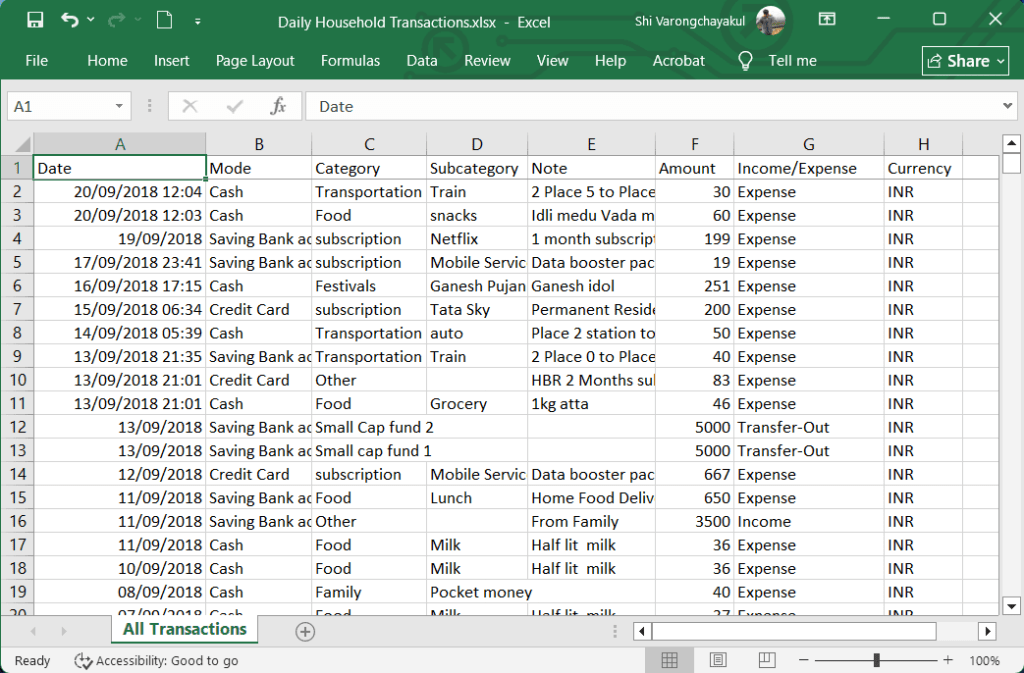
# Import Excel data with read_excel()
all_transactions <- read_excel("Daily Household Transactions.xlsx",
                               sheet = 1)

# View the first few rows
head(all_transactions)

ผลลัพธ์:

# A tibble: 6 × 8
  Date                Mode              Category Subcategory Note  Amount `Income/Expense` Currency
  <dttm>              <chr>             <chr>    <chr>       <chr>  <dbl> <chr>            <chr>   
1 2018-09-20 12:04:08 Cash              Transpo… Train       2 Pl…     30 Expense          INR     
2 2018-09-20 12:03:15 Cash              Food     snacks      Idli…     60 Expense          INR     
3 2018-09-19 00:00:00 Saving Bank acco… subscri… Netflix     1 mo…    199 Expense          INR     
4 2018-09-17 23:41:17 Saving Bank acco… subscri… Mobile Ser… Data…     19 Expense          INR     
5 2018-09-16 17:15:08 Cash              Festiva… Ganesh Puj… Gane…    251 Expense          INR     
6 2018-09-15 06:34:17 Credit Card       subscri… Tata Sky    Perm…    200 Expense          INR

Note: read_excel() มี parametres อื่น ๆ ที่เราสามารถตั้งค่าได้ เช่น:

range: ช่วงข้อมูลที่เราต้องการโหลด
col_names: ชื่อ columns
col_types: ประเภทข้อมูลในแต่ละ column
skip: จำนวน rows ที่เราจะข้ามในการโหลดข้อมูล เช่น เรากำหนด skip = 5, read_excel() จะโหลดข้อมูลตั้งแต่ row ที่ 6 เป็นต้นไป

ดูคู่มือการใช้งาน read_excel() ทั้งหมดได้ที่ read_excel: Read xls and xlsx files.

2️⃣ Package 2. XLConnect

XLConnect เป็น package ที่ช่วยให้เราทำงานกับไฟล์ Excel จาก R ได้โดยตรง

การใช้งาน XLConnect แบ่งได้เป็น 5 กรณี ดังนี้:

โหลดและสำรวจ workbook
โหลดข้อมูลจาก sheet
จัดการ sheet
เพิ่มข้อมูลใน sheet
บันทึก workbook

เราไปดูการใช้งานในแต่ละกรณีกัน

📔 กรณีที่ 1. โหลดและสำรวจ Workbook

ในการเริ่มใช้งาน XLConnect เราจะต้องติดตั้งและโหลด package ก่อน:

# Install
install.packages("XLConnect")

# Load
library(XLConnect)

จากนั้น เราสามารถโหลด Excel เราเข้ามาใน R ได้ด้วย loadWorkbook():

# Load the workbook
workbook <- loadWorkbook("Daily Household Transactions.xlsx")

และดู sheet ทั้งหมดใน workbook ด้วย getSheets():

# List sheets
getSheets(workbook)

ผลลัพธ์:

[1] "All Transactions"

ในตัวอย่าง จะเห็นว่า Excel ของเรามี 1 sheet ได้แก่ “All Transactions”

⬇️ กรณีที่ 2. โหลดข้อมูลจาก sheet

เมื่อเห็นโครงสร้างของไฟล์ Excel แล้ว เราสามารถโหลดข้อมูลจาก sheet ที่ต้องการได้ด้วย readWorksheet():

# Get sheet data
sheet1_data <- readWorksheet(workbook,
                             sheet = "All Transactions")

# Print data
head(sheet1_data)

ผลลัพธ์:

                 Date                  Mode       Category             Subcategory                                     Note Amount Income.Expense Currency
1 2018-09-20 12:04:08                  Cash Transportation                   Train                     2 Place 5 to Place 0     30        Expense      INR
2 2018-09-20 12:03:15                  Cash           Food                  snacks              Idli medu Vada mix 2 plates     60        Expense      INR
3 2018-09-19 00:00:00 Saving Bank account 1   subscription                 Netflix                     1 month subscription    199        Expense      INR
4 2018-09-17 23:41:17 Saving Bank account 1   subscription Mobile Service Provider                        Data booster pack     19        Expense      INR
5 2018-09-16 17:15:08                  Cash      Festivals            Ganesh Pujan                              Ganesh idol    251        Expense      INR
6 2018-09-15 06:34:17           Credit Card   subscription                Tata Sky Permanent Residence - Tata Play recharge    200        Expense      INR

🖐️ กรณีที่ 3. จัดการ Sheet

ในการจัดการ sheet เราสามารถทำได้ 3 อย่าง:

สร้าง sheet ใหม่: createSheet()
เปลี่ยนชื่อ sheet: renameSheet()
ลบ sheet: removeSheet()

ยกตัวอย่างการสร้าง sheet ใหม่:

# Create new sheets
createSheet(workbook,
            name = "New")

# List sheets
getSheets(workbook)

ผลลัพธ์:

[1] "All Transactions" "New"

เปลี่ยนชื่อ sheet:

# Rename the new sheet
renameSheet(workbook,
            sheet = "New",
            newName = "Some Transactions")

# List sheets
getSheets(workbook)

ผลลัพธ์:

[1] "All Transactions"  "Some Transactions"

และลบ sheet ทิ้ง:

# Delete the new sheet
removeSheet(workbook,
            sheet = "Some Transactions")

# List sheets
getSheets(workbook)

ผลลัพธ์:

[1] "All Transactions"

➕ กรณีที่ 4. เพิ่มข้อมูลใน Sheet

เราสามารถใส่ข้อมูลลงใน sheet ได้ด้วย writeWorksheet()

ยกตัวอย่างเช่น เราต้องการเพิ่มข้อมูลสรุปค่าใช้จ่ายตามประเภทการใช้จ่าย

เราจะเริ่มจากสรุปค่าใช้จ่ายตามประเภทโดยใช้ dplyr package:

# Load dplyr
library(dplyr)

# Calculate expense by category
expense_by_cat <- sheet1_data |>
  
  # Filter for expense
  filter(Income.Expense == "Expense") |>
  
  # Group by category
  group_by(Category) |>
  
  # Calculate sum amount
  summarise(Sum = sum(Amount)) |>
    
  # Ungroup
  ungroup() |>
  
  # Sort by category
  arrange(desc(Sum))

# View the results
expense_by_cat

(Note: อ่านเกี่ยวกับการใช้ dplyr ได้ที่นี่)

ผลลัพธ์:

# A tibble: 27 × 2
   Category                  Sum
   <chr>                   <dbl>
 1 Money transfer        606529.
 2 Investment            271858 
 3 Transportation        169054.
 4 Household             161646.
 5 subscription          114588.
 6 Food                   96403.
 7 Public Provident Fund  90000 
 8 Other                  87025.
 9 Family                 78582.
10 Health                 66253.
# ℹ 17 more rows
# ℹ Use `print(n = ...)` to see more rows

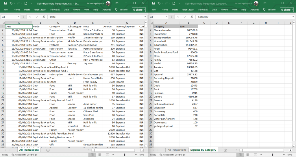
จากนั้น สร้าง sheet ใหม่เพื่อเก็บข้อมูลที่เราได้มา:

# Create a new sheet
createSheet(workbook,
            name = "Expense by Category")

# Add data to "Expense by Catogory" sheet
writeWorksheet(workbook,
               data = expense_by_cat,
               sheet = "Expense by Category")

เมื่อเราเรียกดูข้อมูลจาก “Expense by Catogory” เราจะเห็นข้อมูลแบบนี้:

# Read the sheet
readWorksheet(workbook,
              sheet = "Expense by Category")

ผลลัพธ์:

                Category       Sum
1         Money transfer 606528.90
2             Investment 271858.00
3         Transportation 169053.78
4              Household 161645.58
5           subscription 114587.91
6                   Food  96403.10
7  Public Provident Fund  90000.00
8                  Other  87025.28
9                 Family  78582.20
10                Health  66252.75
11               Tourism  63608.85
12                  Gift  40168.00
13               Apparel  25373.82
14     Recurring Deposit  22000.00
15                  maid  21839.00
16                  Cook  12443.00
17                  Rent  10709.00
18             Festivals   6911.00
19               Culture   4304.36
20                Beauty   4189.00
21      Self-development   2357.00
22             Education    537.00
23              Grooming    400.00
24           Social Life    298.00
25   water (jar /tanker)    148.00
26             Documents    100.00
27      garbage disposal     67.00

💾 กรณีที่ 5. บันทึก Workbook

จนถึงจุดนี้ สิ่งที่เราแก้ไขไปจะยังไม่ถูกบันทึกลงในไฟล์ Excel ของเรา

เราต้องใช้ saveWorkbook() เพื่อบันทึกการเปลี่ยนแปลงทั้งหมดได้

อย่างในตัวอย่าง เราจะบันทึกการเปลี่ยนแปลงทั้งหมดไปที่ workbook ใหม่ชื่อ “Daily Household Transactions (Updated).xlsx”:

# Save the file
saveWorkbook(workbook,
             file = "Daily Household Transactions (Updated).xlsx")

เมื่อเราเปิด working directory ดู เราจะเห็น Excel 2 ไฟล์:

ไฟล์ต้นฉบับ
ไฟล์ที่เราสร้างใหม่

Workbook ต้นฉบับ (ซ้าย) และ workbook ที่เราสร้างใหม่ (ขวา)

💪 Summary

ในบทความนี้ เราได้เรียนรู้วิธีการทำงานกับ Excel ในภาษา R ผ่าน 2 packages ได้แก่:

Package 1. readxl:

Function	For
`read_excel()`	โหลดข้อมูลจาก Excel

Package 2. XLConnect:

Function	For
`loadWorkbook()`	โหลด workbook
`getSheets()`	ดู sheets ใน workbook
`readWorksheet()`	โหลดข้อมูลจาก sheet
`createSheet()`	สร้าง sheet
`renameSheet()`	เปลี่ยนชื่อ sheet
`removeSheet()`	ลบ sheet
`writeWorksheet()`	เพิ่มข้อมูลใน sheet
`saveWorkbook()`	บันทึก workbook

😺 GitHub

ดู code และ Excel ตัวอย่างได้ที่ GitHub

📃 References

Introduction to Importing Data in R

✅ R Book for Psychologists: หนังสือภาษา R สำหรับนักจิตวิทยา

📕 ขอฝากหนังสือเล่มแรกในชีวิตด้วยนะครับ 😆

Correlation
t-tests
ANOVA
Reliability
Factor analysis

แล้วทุกคนจะแปลกใจว่า ทำไมภาษา R ง่ายขนาดนี้ 🙂‍↕️

👉 สนใจดูรายละเอียดหนังสือได้ที่ meb:

ดูรายละเอียดหนังสือ R Book for Psychologists

2025-09-18

4 วิธีการใช้ getSymbols() เพื่อโหลดข้อมูลการเงินในภาษา R — ตัวอย่างการโหลดข้อมูลหุ้น Apple

ในบทความนี้ เราจะมาทำความรู้จักกับ getSymbols() จาก quantmod package ซึ่งใช้โหลดข้อมูลทางการเงิน เช่น ข้อมูลหุ้น และข้อมูลทางเศรษฐกิจ กัน

โดยเราจะไปดู 4 วิธีการใช้งาน ได้แก่:

Basics: การใช้งาน getSymbols() เบื้องต้น
Advanced: การใช้งานขั้นสูง
View columns: การดู column ข้อมูล
Visualise data: การสร้างกราฟข้อมูล

ถ้าพร้อมแล้ว ไปเริ่มกันเลย

💻 Install & Import

ในการใช้งาน getSymbols() เราจะต้องเริ่มจากการติดตั้งและโหลด quantmod package ก่อน แบบนี้:

# Install the packages
install.packages("quantmod")

# Load the packages
library(quantmod)

1️⃣ Basics: 5 Parametres to Know

ในการใช้งานพื้นฐาน getSymbols() มี 5 parametres หลักที่เราควรรู้ ได้แก่:

Symbols: ตัวย่อชื่อข้อมูล
src: แหล่งข้อมูล
auto.assign: ให้โหลด (TRUE) หรือแสดงข้อมูล (FALSE)
env: environment สำหรับโหลดข้อมูล
from และ to: ช่วงเวลาของข้อมูล

เราไปดูวิธีใช้งานแต่ละ parametre กัน

💲 Symbols

ในขั้นแรกของการโหลดข้อมูลการเงินด้วย getSymbols() ให้เราระบุชื่อข้อมูลที่เราต้องการ เช่น:

ข้อมูล	ชื่อข้อมูล
Apple	AAPL
Google	GOOG
Microsoft	MSFT
NVIDIA	NVDA

ในบทความนี้ เราจะลองโหลดข้อมูลหุ้น Apple กัน ซึ่งเราสามารถกำหนด Symbols ได้แบบนี้:

# Import Apple data
getSymbols("AAPL")

เมื่อรันแล้ว เราจะได้ตัวแปรประเภท xts (time series object) ชื่อ AAPL มา ซึ่งเราดูข้อมูลในตัวแปรนี้ได้ด้วย head():

# Print result
head(AAPL)

ผลลัพธ์:

           AAPL.Open AAPL.High AAPL.Low AAPL.Close AAPL.Volume AAPL.Adjusted
2007-01-03  3.081786  3.092143 2.925000   2.992857  1238319600      2.518541
2007-01-04  3.001786  3.069643 2.993571   3.059286   847260400      2.574443
2007-01-05  3.063214  3.078571 3.014286   3.037500   834741600      2.556108
2007-01-08  3.070000  3.090357 3.045714   3.052500   797106800      2.568732
2007-01-09  3.087500  3.320714 3.041071   3.306071  3349298400      2.782115
2007-01-10  3.383929  3.492857 3.337500   3.464286  2952880000      2.915257

จะเห็นได้ว่า นอกจากวันที่แล้ว ข้อมูลเรายังประกอบไปด้วย 6 columns ดังนี้:

Open: ราคาเปิด
High: ราคาสูงสุด
Low: ราคาต่ำสุด
Close: ราคาปิด
Volume: ปริมาณการซื้อขาย
Adjusted: ราคาปรับปรุง

ในกรณีที่เราต้องการโหลดข้อมูลหุ้นหลายตัวพร้อมกัน เราสามารถใช้ character vector ช่วยได้แบบนี้:

# Load multiple instruments
getSymbols(c("AAPL", "GOOGL", "MSFT", "NVDA"))

🏦 src

src ใช้กำหนดแหล่งข้อมูลที่ getSymbols() จะไปดึงข้อมูลมา

โดย default, src ถูกตั้งไว้ให้ดึงข้อมูลจาก Yahoo! Finance ("yahoo")

แสดงว่า เราสามารถเขียน code เพื่อดึงข้อมูล Apple จาก Yahoo! Finance ได้ทั้งแบบนี้:

# Import Apple data
getSymbols("AAPL")

และแบบนี้:

# Import Apple data
getSymbols("AAPL", src = "yahoo")

ทั้งนี้ getSymbols() มีแหล่งข้อมูลอื่น ๆ ให้เราเลือกใช้งานได้ เช่น:

Federal Reserve Economic Data ("FRED")
Oanda ("oanda")

นอกจากแหล่งข้อมูลออนไลน์แล้ว เรายังสามารถโหลดข้อมูลแบบออฟไลน์ได้ เช่น:

CSV ("csv")
RData ("RData")

ยกตัวอย่างเช่น โหลดข้อมูล Apple จาก CSV:

# Load csv data
getSymbols("AAPL", src = "csv")

Note: การโหลดข้อมูล CSV ด้วย getSymbols() มีเงื่อนไข 4 อย่าง ได้แก่:

มีชื่อไฟล์เป็นชื่อหุ้น (เช่น AAPL.csv)
มี header
Column แรกจะต้องเป็น datetime (เช่น 2025-05-25)
Column ที่เหลือควรมีชื่อและข้อมูลดังนี้:
1. Open: ข้อมูลราคาเปิด
2. High: ข้อมูลราคาสูงสุด
3. Low: ข้อมูลราคาต่ำสุด
4. Close: ข้อมูลราคาปิด
5. Volume: ข้อมูลปริมาณการซื้อขาย
6. Adjusted: ข้อมูลราคาปรับปรุง

🏧 auto.assign

auto.assign ใช้กำหนดว่า getSymbols() จะโหลดข้อมูลมาไว้ใน global environment หรือแสดงข้อมูลที่โหลดมาได้

โดย default, auto.assign เป็น TRUE ซึ่งทำให้เราได้ตัวแปรที่เก็บข้อมูลการเงินมาไว้ใน global environment ของเรา โดยไม่ต้องกำหนดตัวแปรเอง

ทั้งนี้ ในกรณีที่เราต้องการกำหนดตัวแปรเอง ให้เราเปลี่ยน auto.assign เป็น FALSE แบบนี้:

# Set auto.assign to FALSE to assign to custom variable
apple_data <- getSymbols("AAPL", auto.assign = FALSE)

ถ้าเรากำหนดให้ auto.assign = FALSE โดยไม่จัดเก็บไว้ในตัวแปร getSymbols() จะแสดงข้อมูลใน console ของเรา:

# Set auto.assign to FALSE without variable assignment
getSymbols("AAPL", auto.assign = FALSE)

ผลลัพธ์:

            AAPL.Open  AAPL.High   AAPL.Low AAPL.Close AAPL.Volume AAPL.Adjusted
2007-01-03   3.081786   3.092143   2.925000   2.992857  1238319600      2.518541
2007-01-04   3.001786   3.069643   2.993571   3.059286   847260400      2.574442
2007-01-05   3.063214   3.078571   3.014286   3.037500   834741600      2.556108
2007-01-08   3.070000   3.090357   3.045714   3.052500   797106800      2.568732
2007-01-09   3.087500   3.320714   3.041071   3.306071  3349298400      2.782115
2007-01-10   3.383929   3.492857   3.337500   3.464286  2952880000      2.915257
2007-01-11   3.426429   3.456429   3.396429   3.421429  1440252800      2.879192
2007-01-12   3.378214   3.395000   3.329643   3.379286  1312690400      2.843727
2007-01-16   3.417143   3.473214   3.408929   3.467857  1244076400      2.918262
2007-01-17   3.484286   3.485714   3.386429   3.391071  1646260000      2.853645
       ...                                                                      
2025-06-05 203.500000 204.750000 200.149994 200.630005    55126100    200.630005
2025-06-06 203.000000 205.699997 202.050003 203.919998    46607700    203.919998
2025-06-09 204.389999 206.000000 200.020004 201.449997    72862600    201.449997
2025-06-10 200.600006 204.350006 200.570007 202.669998    54672600    202.669998
2025-06-11 203.500000 204.500000 198.410004 198.779999    60989900    198.779999
2025-06-12 199.080002 199.679993 197.360001 199.199997    43904600    199.199997
2025-06-13 199.729996 200.369995 195.699997 196.449997    51447300    196.449997
2025-06-16 197.300003 198.690002 196.559998 198.419998    43020700    198.419998
2025-06-17 197.199997 198.389999 195.210007 195.639999    38856200    195.639999
2025-06-18 195.940002 197.570007 195.070007 196.580002    45350400    196.580002

🌲 env

env ใช้กำหนด environment ที่ใช้เก็บข้อมูล ซึ่งโดย default, getSymbols() จะโหลดข้อมูลไว้ใน global environment

ในการใช้ env กำหนด environment ที่ต้องการ เราจะต้องเริ่มจากสร้าง environment ขึ้นมาก่อนด้วย new.env():

# Create a new environment
my_env <- new.env()

จากนั้น โหลดข้อมูลเข้าไปใน environment ใหม่:

# Load data into the environment
getSymbols("AAPL", env = my_env)

เราสามารถดูตัวแปรที่เก็บไว้ใน environment ได้ด้วย ls():

# List all variables in environment
ls(envir = my_env)

และดูข้อมูลได้ด้วย $ เช่น:

# Show Apple data
head(my_env$AAPL)

ผลลัพธ์:

           AAPL.Open AAPL.High AAPL.Low AAPL.Close AAPL.Volume AAPL.Adjusted
2007-01-03  3.081786  3.092143 2.925000   2.992857  1238319600      2.518541
2007-01-04  3.001786  3.069643 2.993571   3.059286   847260400      2.574442
2007-01-05  3.063214  3.078571 3.014286   3.037500   834741600      2.556109
2007-01-08  3.070000  3.090357 3.045714   3.052500   797106800      2.568732
2007-01-09  3.087500  3.320714 3.041071   3.306071  3349298400      2.782115
2007-01-10  3.383929  3.492857 3.337500   3.464286  2952880000      2.915256

📆 from, to

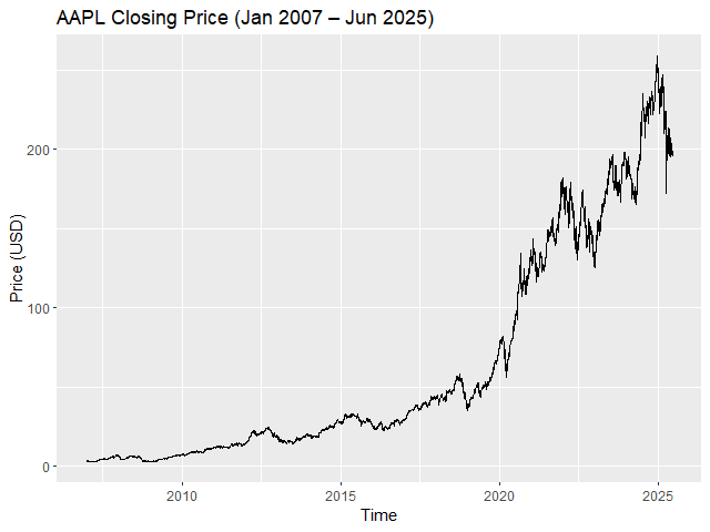
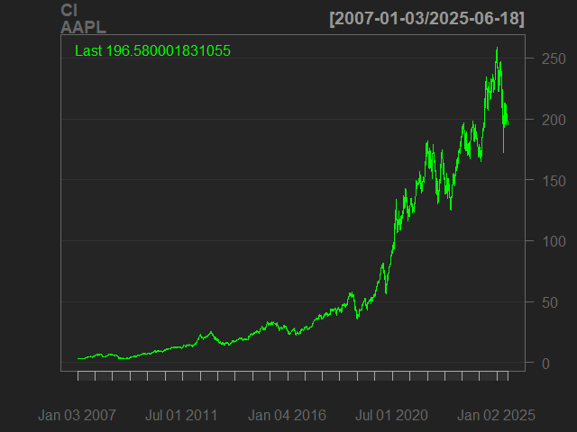
from ใช้กำหนดวันแรกของข้อมูล และ to กำหนดวันสุดท้ายของข้อมูล

ยกตัวอย่างเช่น เราต้องการโหลดข้อมูล Apple ในเดือนพฤษภาคม 2025:

# Load data for May 2025
apple_data_2025_05 = getSymbols("AAPL",
                                auto.assign = FALSE,
                                from = "2025-05-01",
                                to = "2025-05-31")

# Print results
print("First three records:")
head(apple_data_2025_05, n = 3)
print("------------------------------------------------------------------------------")
print("Last three records:")
tail(apple_data_2025_05, n = 3)

ผลลัพธ์:

First three records:
           AAPL.Open AAPL.High AAPL.Low AAPL.Close AAPL.Volume AAPL.Adjusted
2025-05-01    209.08    214.56   208.90     213.32    57365700      213.0406
2025-05-02    206.09    206.99   202.16     205.35   101010600      205.0811
2025-05-05    203.10    204.10   198.21     198.89    69018500      198.6295
------------------------------------------------------------------------------
Last three records:
           AAPL.Open AAPL.High AAPL.Low AAPL.Close AAPL.Volume AAPL.Adjusted
2025-05-28    200.59    202.73   199.90     200.42    45339700        200.42
2025-05-29    203.58    203.81   198.51     199.95    51396800        199.95
2025-05-30    199.37    201.96   196.78     200.85    70819900        200.85

Note: ตลาดหุ้นวันสุดท้ายของเดือนพฤษภาคม 2025 คือ 30 พฤษภาคม ทำให้ข้อมูลสิ้นสุด ณ วันที่ 30

2️⃣ Advanced: Set Defaults

จะเห็นว่า getSymbols() การตั้งค่าที่หลากหลาย

ทั้งนี้ quantmod มี 6 functions ที่ใช้ร่วมกับ getSymbols() เพื่อช่วยลดขั้นตอนในการตั้งค่าต่าง ๆ ได้แก่:

getDefaults() และ setDefaults()
getSymbolLookup() และ setSymbolLookup()
saveSymbolLookup() และ loadSymbolLookup()

เราไปดูวิธีการใช้งานทั้ง 6 functions กัน

🌍 getDefaults(), setDefaults()

getDefaults() ใช้สำหรับดูค่า default ของ getSymbols()

ส่วน setDefaults() ใช้สำหรับกำหนดค่า default

ยกตัวอย่างเช่น เราต้องการกำหนด:

src จาก "yahoo" เป็น "FRED"
auto.assign จาก TRUE เป็น FALSE

เราสามารถทำได้แบบนี้:

# Get defaults before changing
print("Defaults (before):")
getDefaults(getSymbols)

# Set defaults
setDefaults(getSymbols,
            src = "FRED",
            auto.assign = FALSE)
 
# Get defaults after changing
print("Defaults (after):")
getDefaults(getSymbols)

ผลลัพธ์:

Defaults (before):
NULL

Defaults (after):
$src
[1] "'FRED'"

$auto.assign
[1] FALSE

ตอนนี้ ถ้าเราเรียกใช้ getSymbols() โดยไม่กำหนด src และ auto.assign ทั้งสอง arguments นี้จะเป็น "FRED" และ FALSE ตามลำดับ

ถ้าเราต้องการ reset ค่า default ให้เราใส่ NULL ใน setDefaults():

# Reset defaults
setDefaults(getSymbols,
            src = NULL,
            auto.assign = NULL)

# Check defaults after resetting
print("Defaults (reset):")
getDefaults(getSymbols)

ผลลัพธ์:

Defaults (reset):
NULL

💹 setSymbolLookup(), getSymbolLookup()

getSymbolLookup() และ setSymbolLookup() ทำงานเหมือนกับ getDefaults() และ setDefaults() แต่เป็นการตั้งค่า default สำหรับข้อมูลแต่ละตัว (แทนระดับ global) ภายใน session เท่านั้น

ยกตัวอย่างเช่น เราต้องการกำหนดให้ดึงข้อมูลหุ้น Google มาจาก Google Finance:

# Set default for Google
setSymbolLookup(GOOG = list(src = "google"))

# Get new defaults
getSymbolLookup()

ผลลัพธ์:

$GOOG
$GOOG$src
[1] "google"

Note: Google Finance หยุดให้ข้อมูลกับ quantmod เมื่อปี 2018 ทำให้ตอนนี้ เราไม่สามารถใช้ src = "google" ได้อีก

เราสามารถ reset ค่า default ได้โดยใส่ NULL เหมือนเดิม:

# Reset defaults
setSymbolLookup(NULL)

# Get defaults after resetting
getSymbolLookup()

ผลลัพธ์:

named list()

💾 saveSymbolLookup(), loadSymbolLookup()

ค่าที่เราใช้ setSymbolLookup() กำหนดจะถูก reset ทุกครั้งที่เราปิด session ไป

ถ้าเราต้องการเก็บค่าเพื่อไปใช้ใน session อื่น เราสามารถใช้ saveSymbolLookup() และ loadSymbolLookup() ช่วยได้:

saveSymbolLookup() บันทึกค่าเก็บไว้ในไฟล์ RDS
loadSymbolLookup() โหลดค่าที่เก็บไว้ใน RDS

ตัวอย่าง code:

# Save defaults
saveSymbolLookup(file = "symbols.rds")

# Load defaults
loadSymbolLookup(file = "symbols.rds")

3️⃣ View Columns

หลังจากเราโหลดข้อมูลมาแล้ว เราสามารถดูข้อมูลแต่ละ column ได้ด้วย 7 functions หลัก ดังนี้:

No.	Function	For
1	`Op()`	ราคาเปิด
2	`Hi()`	ราคาสูงสุด
3	`Lo()`	ราคาต่ำสุด
4	`Cl()`	ราคาปิด
5	`Ad()`	ราคาปรับปรุง
6	`Vo()`	ปริมาณการซื้อขาย
7	`OHLC()`	ราคาเปิด, สูงสุด, ต่ำสุด, และราคาปิด

ตัวอย่างเช่น ดูราคาเปิด:

# Get opening price
Op(AAPL)

ผลลัพธ์:

            AAPL.Open
2007-01-03   3.081786
2007-01-04   3.001786
2007-01-05   3.063214
2007-01-08   3.070000
2007-01-09   3.087500
2007-01-10   3.383929
2007-01-11   3.426429
2007-01-12   3.378214
2007-01-16   3.417143
2007-01-17   3.484286
       ...           
2025-06-05 203.500000
2025-06-06 203.000000
2025-06-09 204.389999
2025-06-10 200.600006
2025-06-11 203.500000
2025-06-12 199.080002
2025-06-13 199.729996
2025-06-16 197.300003
2025-06-17 197.199997
2025-06-18 195.940002

ดูราคาสูงสุด:

# Get highest price
Hi(AAPL)

ผลลัพธ์:

            AAPL.High
2007-01-03   3.092143
2007-01-04   3.069643
2007-01-05   3.078571
2007-01-08   3.090357
2007-01-09   3.320714
2007-01-10   3.492857
2007-01-11   3.456429
2007-01-12   3.395000
2007-01-16   3.473214
2007-01-17   3.485714
       ...           
2025-06-05 204.750000
2025-06-06 205.699997
2025-06-09 206.000000
2025-06-10 204.350006
2025-06-11 204.500000
2025-06-12 199.679993
2025-06-13 200.369995
2025-06-16 198.690002
2025-06-17 198.389999
2025-06-18 197.570007

ดูราคาต่ำสุด:

# Get lowest price
Lo(AAPL)

ผลลัพธ์:

             AAPL.Low
2007-01-03   2.925000
2007-01-04   2.993571
2007-01-05   3.014286
2007-01-08   3.045714
2007-01-09   3.041071
2007-01-10   3.337500
2007-01-11   3.396429
2007-01-12   3.329643
2007-01-16   3.408929
2007-01-17   3.386429
       ...           
2025-06-05 200.149994
2025-06-06 202.050003
2025-06-09 200.020004
2025-06-10 200.570007
2025-06-11 198.410004
2025-06-12 197.360001
2025-06-13 195.699997
2025-06-16 196.559998
2025-06-17 195.210007
2025-06-18 195.070007

ดูราคาปิด:

# Get closing price
Cl(AAPL)

ผลลัพธ์:

           AAPL.Close
2007-01-03   2.992857
2007-01-04   3.059286
2007-01-05   3.037500
2007-01-08   3.052500
2007-01-09   3.306071
2007-01-10   3.464286
2007-01-11   3.421429
2007-01-12   3.379286
2007-01-16   3.467857
2007-01-17   3.391071
       ...           
2025-06-05 200.630005
2025-06-06 203.919998
2025-06-09 201.449997
2025-06-10 202.669998
2025-06-11 198.779999
2025-06-12 199.199997
2025-06-13 196.449997
2025-06-16 198.419998
2025-06-17 195.639999
2025-06-18 196.580002

ดูราคาปรับปรุง:

# Get adjusted price
Ad(AAPL)

ผลลัพธ์:

           AAPL.Adjusted
2007-01-03      2.518541
2007-01-04      2.574442
2007-01-05      2.556109
2007-01-08      2.568732
2007-01-09      2.782116
2007-01-10      2.915256
2007-01-11      2.879192
2007-01-12      2.843727
2007-01-16      2.918261
2007-01-17      2.853645
       ...              
2025-06-05    200.630005
2025-06-06    203.919998
2025-06-09    201.449997
2025-06-10    202.669998
2025-06-11    198.779999
2025-06-12    199.199997
2025-06-13    196.449997
2025-06-16    198.419998
2025-06-17    195.639999
2025-06-18    196.580002

ดูปริมาณการซื้อขาย:

# Get volume
Vo(AAPL)

ผลลัพธ์:

           AAPL.Volume
2007-01-03  1238319600
2007-01-04   847260400
2007-01-05   834741600
2007-01-08   797106800
2007-01-09  3349298400
2007-01-10  2952880000
2007-01-11  1440252800
2007-01-12  1312690400
2007-01-16  1244076400
2007-01-17  1646260000
       ...            
2025-06-05    55126100
2025-06-06    46607700
2025-06-09    72862600
2025-06-10    54672600
2025-06-11    60989900
2025-06-12    43904600
2025-06-13    51447300
2025-06-16    43020700
2025-06-17    38856200
2025-06-18    45350400

ดูราคาเปิด, สูงสุด, ต่ำสุด, และราคาปิด:

# Get all price
OHLC(AAPL)

ผลลัพธ์:

            AAPL.Open  AAPL.High   AAPL.Low AAPL.Close
2007-01-03   3.081786   3.092143   2.925000   2.992857
2007-01-04   3.001786   3.069643   2.993571   3.059286
2007-01-05   3.063214   3.078571   3.014286   3.037500
2007-01-08   3.070000   3.090357   3.045714   3.052500
2007-01-09   3.087500   3.320714   3.041071   3.306071
2007-01-10   3.383929   3.492857   3.337500   3.464286
2007-01-11   3.426429   3.456429   3.396429   3.421429
2007-01-12   3.378214   3.395000   3.329643   3.379286
2007-01-16   3.417143   3.473214   3.408929   3.467857
2007-01-17   3.484286   3.485714   3.386429   3.391071
       ...                                            
2025-06-05 203.500000 204.750000 200.149994 200.630005
2025-06-06 203.000000 205.699997 202.050003 203.919998
2025-06-09 204.389999 206.000000 200.020004 201.449997
2025-06-10 200.600006 204.350006 200.570007 202.669998
2025-06-11 203.500000 204.500000 198.410004 198.779999
2025-06-12 199.080002 199.679993 197.360001 199.199997
2025-06-13 199.729996 200.369995 195.699997 196.449997
2025-06-16 197.300003 198.690002 196.559998 198.419998
2025-06-17 197.199997 198.389999 195.210007 195.639999
2025-06-18 195.940002 197.570007 195.070007 196.580002

4️⃣ Visualise Data

สุดท้าย เราสามารถสร้างกราฟเพื่อสำรวจข้อมูล โดยใช้ 2 functions ได้แก่:

autoplot() จาก ggplot2 package
chartSeries() จาก quantmod package

ยกตัวอย่างเช่น สำรวจราคาปิดของ Apple:

# Import ggplots
library(ggplot2)

# Visualise with autoplot()
autoplot(Cl(AAPL),
         ts.colour = "darkgreen") +

  # Add text
  labs(title = "AAPL Closing Price (Jan 2007 – Jun 2025)",
       x = "Time",
       y = "Price (USD)")

ผลลัพธ์:

# Visualise with chartSeries()
chartSeries(Cl(AAPL))

ผลลัพธ์:

💪 Summary

ในบทความนี้ เราได้ดูวิธีการทำงานกับ getSymbols() เพื่อโหลดข้อมูลจากการเงินจากแหล่งต่าง ๆ กัน

ตอนนี้ เรารู้จักกับ 5 parametres หลักของ getSymbols():

Symbols
src
auto.assign
env
from และ to

วิธีตั้งค่า default ด้วย 3 คู่ functions:

getDefaults() และ setDefaults()
getSymbolLookup() และ setSymbolLookup()
saveSymbolLookup() และ loadSymbolLookup()

วิธีดูข้อมูลด้วย 7 functions:

Op()
Hi()
Lo()
Cl()
Ad()
Vo()
OHLC()

และสุดท้าย วิธีสร้างกราฟด้วย 2 functions:

autoplot()
chartSeries()

😺 GitHub

ดู code ทั้งหมดในบทความนี้ได้ที่ GitHub

📃 References

✅ R Book for Psychologists: หนังสือภาษา R สำหรับนักจิตวิทยา

📕 ขอฝากหนังสือเล่มแรกในชีวิตด้วยนะครับ 😆

Correlation
t-tests
ANOVA
Reliability
Factor analysis

แล้วทุกคนจะแปลกใจว่า ทำไมภาษา R ง่ายขนาดนี้ 🙂‍↕️

👉 สนใจดูรายละเอียดหนังสือได้ที่ meb:

ดูรายละเอียดหนังสือ R Book for Psychologists

2025-08-28

7 วิธีทำงานกับ time series data ในภาษา R: Base R, lubridate, และ zoo packages — ตัวอย่างการวิเคราะห์ราคา Bitcoin

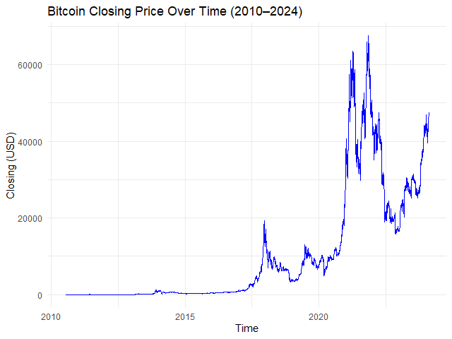
ในบทความนี้ เราจะมาเรียนรู้ 7 วิธีการทำงานกับ time series data หรือข้อมูลที่จัดเรียงด้วยเวลา ในภาษา R ผ่านการทำงานกับ Bitcoin Historical Data ซึ่งมีข้อมูล Bitcoin ในช่วงปี ค.ศ. 2010–2024 กัน:

Converting: การแปลงข้อมูลเป็น datetime และ time series
Missing values: การจัดการ missing values ใน time series data
Plotting: การสร้างกราฟ time series data
Subsetting: การเลือกข้อมูลจาก time series data
Aggregating: การสรุป time series data
Rolling window: การทำ rolling window
Expanding window: การทำ expanding window

ถ้าพร้อมแล้วไปเริ่มกันเลย

🏁 Getting Started

ในการเริ่มทำงานกับ time series ในภาษา R เราจะเริ่มต้นจาก 2 อย่าง ได้แก่:

Install and load packages
Load dataset

1️⃣ Install & Load Packages

ในภาษา R เรามี 3 packages ที่ใช้ทำงานกับ time series data บ่อย ๆ ได้แก่:

Base R packages ที่มาพร้อมกับภาษา R
lubridate: ใช้แปลงข้อมูลและจัด format ของ date-time data
zoo: ใช้ทำงานกับ time series data

ในการเริ่มต้นใช้งาน เราจะติดตั้ง packages เหล่านี้กัน:

# Install packages
install.packages("lubridate"
install.packages("zoo")
install.packages("ggplot2") # for data visualisation

จากนั้น เรียกใช้งาน packages:

# Load packages
library(lubridate)
library(zoo)
library(ggplot2) # for data visualisation

Note: เราเพิ่ม ggplot2 เข้ามาด้วย เพื่อช่วยในการสร้างกราฟในภายหลัง

2️⃣ Load Dataset

หลังติดตั้งและเรียกใช้งาน packages เราจะโหลด Bitcoin Historical Data (ดาวน์โหลดไฟล์ได้ที่ Kaggle) เข้ามาใน environment:

# Load the dataset
btc <- read.csv("btc_hist_2010-2024.csv")

จากนั้น เราสามารถสำรวจข้อมูลได้ด้วย head() และ str():

## View the first 6 rows
head(btc)

## View the structure
str(btc)

ผลลัพธ์ของ head():

          Date    Price     Open     High      Low   Vol. Change..
1 Feb 09, 2024 47,545.4 45,293.3 47,710.2 45,254.2 86.85K    4.97%
2 Feb 08, 2024 45,293.3 44,346.2 45,579.2 44,336.4 66.38K    2.15%
3 Feb 07, 2024 44,339.8 43,088.4 44,367.9 42,783.5 48.57K    2.91%
4 Feb 06, 2024 43,087.7 42,697.6 43,375.5 42,566.8 33.32K    0.91%
5 Feb 05, 2024 42,697.2 42,581.4 43,532.2 42,272.5 39.26K    0.27%
6 Feb 04, 2024 42,581.4 43,006.2 43,113.2 42,379.4 20.33K   -0.99%

ผลลัพธ์ของ str():

'data.frame':	4955 obs. of  7 variables:
 $ Date    : chr  "Feb 09, 2024" "Feb 08, 2024" "Feb 07, 2024" "Feb 06, 2024" ...
 $ Price   : chr  "47,545.4" "45,293.3" "44,339.8" "43,087.7" ...
 $ Open    : chr  "45,293.3" "44,346.2" "43,088.4" "42,697.6" ...
 $ High    : chr  "47,710.2" "45,579.2" "44,367.9" "43,375.5" ...
 $ Low     : chr  "45,254.2" "44,336.4" "42,783.5" "42,566.8" ...
 $ Vol.    : chr  "86.85K" "66.38K" "48.57K" "33.32K" ...
 $ Change..: chr  "4.97%" "2.15%" "2.91%" "0.91%" ...

จากผลลัพธ์ เราจะเห็นว่า Bitcoin Historical Data มี 7 columns ด้วยกัน ได้แก่:

No.	Column	Description
1	`Date`	วันที่
2	`Close`	ราคาปิด (USD)
3	`Open`	ราคาเปิด (USD)
4	`High`	ราคาสูงสุด (USD)
5	`Low`	ราคาต่ำสุด (USD)
6	`Vol.`	ปริมาณการซื้อขาย
7	`Change..`	การเปลี่ยนแปลงราคาจากวันก่อน (คิดเป็น %)

นอกจากนี้ เราจะเห็นได้ว่า ทุก column เป็น character ซึ่งเราจะต้องแปลงให้เป็นประเภทข้อมูลที่ถูกต้องก่อน ซึ่งเราสามารถทำได้ดังนี้:

สร้าง copy ของ btc
เปลี่ยนชื่อ column (เพื่อให้ง่ายต่อการทำงาน)
เปลี่ยน format ข้อมูลของ price และ volume
แปลงประเภทข้อมูลจาก character เป็น numeric

# Clean the dataset

## Make a copy of the dataset
btc_cleaned <- btc

## Rename columns

### Create new column names
new_col_names <- c("date",
                   "close", "open",
                   "high", "low",
                   "volume", "change")

### Rename
colnames(btc_cleaned) <- new_col_names

### Check the results
str(btc_cleaned)

## Convert data types

### Specify the columns to clean
cols_to_clean <- c("close", "open",
                   "high", "low")

### Remove comma
for (col in cols_to_clean) {
  btc_cleaned[[col]] <- gsub(",",
                             "",
                             btc_cleaned[[col]])
}

### Remove "K"
btc_cleaned$volume <- gsub("K",
                           "",
                           btc_cleaned$volume)

### Remove "%"
btc_cleaned$change <- gsub("%",
                           "",
                           btc_cleaned$change)

### Specify columns to convert to numeric
cols_to_num <- colnames(btc_cleaned[, -1])

### Convert data type to numeric
for (col in cols_to_num) {
  btc_cleaned[[col]] <- as.numeric(btc_cleaned[[col]])
}

### Check the results
str(btc_cleaned)

ผลลัพธ์:

'data.frame':	4955 obs. of  7 variables:
 $ date  : chr  "Feb 09, 2024" "Feb 08, 2024" "Feb 07, 2024" "Feb 06, 2024" ...
 $ close : num  47545 45293 44340 43088 42697 ...
 $ open  : num  45293 44346 43088 42698 42581 ...
 $ high  : num  47710 45579 44368 43376 43532 ...
 $ low   : num  45254 44336 42784 42567 42273 ...
 $ volume: num  86.8 66.4 48.6 33.3 39.3 ...
 $ change: num  4.97 2.15 2.91 0.91 0.27 -0.99 -0.44 0.26 1.18 -0.85 ...

ตอนนี้ ทุก column (ยกเว้น date) ถูกเปลี่ยนให้เป็น numeric เรียบร้อยแล้ว และชุดข้อมูลก็พร้อมจะถูกนำไปใช้งานต่อแล้ว

🔄️ Converting

เรามาดูวิธีแรกในการทำงานกับ time series data กัน นั่นคือ:

การแปลงข้อมูลให้เป็น datetime
การแปลงข้อมูลให้เป็น time series

1️⃣ การแปลงข้อมูลให้เป็น Datetime

ในการทำงานกับ time series data เราจะต้องแปลงข้อมูลประเภทอื่น ๆ เช่น character และ numeric ให้เป็น datetime ก่อน เช่น date (เช่น “Feb 09, 2024”) ใน Bitcoin dataset

เราสามารถแปลงข้อมูลจาก character เป็น Date ได้ 2 วิธี ดังนี้:

วิธีที่ 1. ใช้ as.Date() ซึ่งเป็น base R function และต้องการ input 2 อย่าง ได้แก่:

x: ข้อมูลที่ต้องการแปลงเป็น Date
format: format ของวันเวลาของข้อมูลต้นทาง (เช่น วัน-เดือน-ปี, ปี-เดือน-วัน, เดือน-วัน-ปี)

# Convert `date` to Date
btc_cleaned$date <- as.Date(btc_cleaned$date,
                            format = "%b %d, %Y")

Note: ศึกษาการกำหนด format ได้ที่ strptime: Date-time Conversion Functions to and from Character และ Date Formats in R

วิธีที่ 2. ใช้ as_date() จาก lubridate ซึ่งเป็นที่นิยมมากกว่า as.Date() เพราะ as_date() แปลงข้อมูลให้อัตโนมัติ โดยเราไม่ต้องกำหนด format ให้:

# Convert `date` to Date
btc_cleaned$date <- as_date(btc_cleaned$date)

จากตัวอย่าง จะเห็นได้ว่า as_date() ใช้งานง่ายกว่า as.Date()

ทั้งนี้ ทั้งสองวิธีให้ผลลัพธ์เหมือนกัน คือ แปลง character เป็น Date ซึ่งเราสามารถเช็กผลลัพธ์ได้ด้วย str():

# Check the results
str(btc_cleaned)

ผลลัพธ์:

'data.frame':	4955 obs. of  7 variables:
 $ date  : Date, format: "2024-02-09" "2024-02-08" "2024-02-07" ...
 $ close : num  47545 45293 44340 43088 42697 ...
 $ open  : num  45293 44346 43088 42698 42581 ...
 $ high  : num  47710 45579 44368 43376 43532 ...
 $ low   : num  45254 44336 42784 42567 42273 ...
 $ volume: num  86.8 66.4 48.6 33.3 39.3 ...
 $ change: num  4.97 2.15 2.91 0.91 0.27 -0.99 -0.44 0.26 1.18 -0.85 ...

จะเห็นได้ว่า ตอนนี้ price เปลี่ยนเป็นจาก character เป็น Date เรียบร้อยแล้ว

2️⃣ การแปลงข้อมูลให้เป็น Time Series

นอกจากการแปลงข้อมูลบางส่วนให้เป็น datetime แล้ว เรายังต้องการแปลง dataset จาก data frame ให้เป็น time series เพื่อมี index ของข้อมูล เป็น datetime

ในภาษา R เรามี time series 2 ประเภทหลัก ได้แก่:

ts ของ base R ซึ่งเหมาะกับข้อมูลที่มีความถี่คงที่ (เช่น ข้อมูลมีระยะห่างกัน 1 วัน)
zoo จาก zoo package ซึ่งเหมาะกับข้อมูลที่มีความถี่ไม่คงที่ (เช่น บางข้อมูลห่างกัน 1 วัน และบางข้อมูลห่างกัน 1 เดือน)

ในตัวอย่าง Bitcoin เราจะแปลง dataset ให้เป็น zoo กัน:

# Convert data frame to zoo object

## Convert
btc_zoo <- zoo(btc_cleaned[, -1],
               order.by = btc_cleaned$date)

## Check the results
head(btc_zoo)

ผลลัพธ์:

           close open high low volume change
2010-07-18   0.1  0.0  0.1 0.1   0.08      0
2010-07-19   0.1  0.1  0.1 0.1   0.57      0
2010-07-20   0.1  0.1  0.1 0.1   0.26      0
2010-07-21   0.1  0.1  0.1 0.1   0.58      0
2010-07-22   0.1  0.1  0.1 0.1   2.16      0
2010-07-23   0.1  0.1  0.1 0.1   2.40      0

จะเห็นได้ว่า datetime ถูกเปลี่ยนให้เป็น index ของข้อมูลแล้ว

🤷‍♂️ Missing Values

ในบางครั้ง เราอาจมี time series data ที่มีข้อมูลขาดหายไป ซึ่งเราอาจต้องการแทนที่ด้วยค่าบางอย่าง

ในตัวอย่าง Bitcoin dataset เรามี missing values อยู่ใน volume ซึ่งเราสามารถเช็กได้ด้วย colSums() และ is.na() แบบนี้:

# Count the missing values in each column
colSums(is.na(btc_zoo))

ผลลัพธ์:

 close   open   high    low volume change 
     0      0      0      0    271      0

zoo package มี 3 functions ที่ช่วยให้เราแทนค่า missing values ได้ ดังนี้:

No.	Function	Description
1	`na.fill()`	แทนค่าด้วยค่าที่เรากำหนด
2	`na.locf()`	แทนค่าตามค่าของข้อมูลที่มาก่อนหน้า
3	`na.approx()`	แทนค่าด้วยตามข้อมูลที่มาก่อนและหลัง missing values

สำหรับ Bitcoin dataset เราจะใช้ na.approx() เนื่องจากข้อมูล Bitcoin มีความผันผวนและการแทนค่าแบบยืดหยุ่นจะดีกว่าการแทนค่าแบบกำหนดตายตัว:

# Impute with na.approx()
btc_zoo <- na.approx(btc_zoo)

# Check the results
colSums(is.na(btc_zoo))

ผลลัพธ์:

 close   open   high    low volume change 
     0      0      0      0      0      0

ตอนนี้ missing values ถูกแทนค่าเรียบร้อย

📈 Plotting

การสร้างกราฟสามารถช่วยให้เราเข้าใจ time series data ได้ง่ายขึ้น

เราสามารถทำได้ง่าย ๆ ด้วย autoplot.*() เช่น autoplot.ts() และ autplot.zoo()

ใน Bitcoin dataset เราสามารถสร้างกราฟราคาปิดของ Bitcoin ในช่วง 2010**–**2024 ได้ด้วย autoplot.zoo() แบบนี้:

# Plot the time series
autoplot.zoo(btc_zoo[, "close"]) +
  
  ## Adjust line colour
  geom_line(color = "blue") +
  
  ## Add title and labels
  labs(title = "Bitcoin Closing Price Over Time (2010–2024)",
       x = "Time",
       y = "Closing Price (USD)") +
  
  ## Use minimal theme
  theme_minimal()

ผลลัพธ์:

Note: ในตัวอย่าง เราใช้ ggplot2 ช่วยตกแต่งกราฟให้เข้าใจง่ายขึ้น, สำหรับคนที่สนใจ สามารถศึกษาการใช้ ggplot2 ได้ที่ วิธีใช้ ggplot2 เพื่อสร้างกราฟอย่างมืออาชีพระดับโลก แบบ BBC และ Financial Times ในภาษา R — ตัวอย่างการสำรวจข้อมูลเพนกวินจาก palmerpenguins

✂️ Subsetting

ในการทำงานกับ time series data เราอาจต้องการตัดแบ่งข้อมูลบางส่วนมาเพื่อสำรวจการเปลี่ยนแปลงของข้อมูลในช่วงเวลาที่ต้องการ

ยกตัวอย่างเช่น เราอยากจะสำรวจการเปลี่ยนแปลงราคาปิดของ Bitcoin ในช่วง Crypto Winter (Nov 2021 – Dec 2022)

ในภาษา R เราสามารถตัดแบ่ง time series ได้ 3 วิธี ได้แก่:

window()
Boolean masking
Specific date

1️⃣ window()

window() เป็น base R function ซึ่งช่วยเราเลือกช่วงเวลาได้ด้วย input 3 อย่าง:

x: time series data
start: วันเริ่มต้น (inclusive)
end: วันสิ้นสุด (inclusive)

เราสามารถใช้ window() สร้างกราฟได้แบบนี้:

# Subset
btc_winter_1 <- window(x = btc_zoo,
                       start = as.Date("2021-11-01"),
                       end = as.Date("2022-12-31"))

# Plot the results
autoplot.zoo(btc_winter_1[, "close"]) +
  
  ## Adjust line colour
  geom_line(color = "blue") +
  
  ## Add title and labels
  labs(title = "Bitcoin Closing Price During the Crypto Winter (2021–2022)",
       x = "Time",
       y = "Closing (USD)") +
  
  ## Use minimal theme
  theme_minimal()

ผลลัพธ์:

2️⃣ Boolean Masking

นอกจาก window() แล้ว เราสามารถเลือกช่วงเวลาด้วยการสร้าง Boolean mask ขึ้นมา แบบนี้:

# Create a Boolean masking
crypto_winter_index <- 
  index(btc_zoo) >= "2021-11-01" &
  index(btc_zoo) <= "2022-12-31"

# Subset
btc_winter_2 <- btc_zoo[crypto_winter_index, ]

# Plot the results
autoplot.zoo(btc_winter_2[, "close"]) +  
  
  ## Adjust line colour
  geom_line(color = "blue") +
  
  ## Add title and labels
  labs(title = "Bitcoin Closing Price During the Crypto Winter (2021–2022)",
       x = "Time",
       y = "Closing (USD)") +
  
  ## Use minimal theme
  theme_minimal()

ผลลัพธ์:

จะเห็นว่า กราฟของ Boolean masking เหมือนกับการใช้ window()

3️⃣ Specific Date

ในกรณีที่เราต้องการเลือกวันแทนช่วงเวลา (เช่น ดูข้อมูล Bitcoin เมื่อเกิด halving ครั้งแรก) เราสามารถเขียนภาษา R ได้แบบนี้:

# Subset
btc_first_halving <- btc_zoo["2012-11-28"]

# Print the result
btc_first_halving

ผลลัพธ์:

           close open high  low volume change
2012-11-28  12.4 12.2 12.4 12.1  30.69   1.23

🧮 Aggregating

ในภาษา R เราสามารถสรุปข้อมูล time series data (เช่น หาค่าเฉลี่ย) ได้ด้วย apply.*() จาก zoo package:

Function	Description
`apply.daily()`	สรุปข้อมูลรายวัน
`apply.weekly()`	สรุปข้อมูลรายสัปดาห์
`apply.quarterly()`	สรุปข้อมูลรายไตรมาส
`apply.yearly()`	สรุปข้อมูลรายปี

โดย apply.*() ต้องการ input 2 อย่าง คือ:

x: time series data
FUN: การสรุปข้อมูล (เช่น mean, median, max, min)

ยกตัวอย่างเช่น หาค่าเฉลี่ยราคาปิดของ Bitcoin ในแต่ละปี:

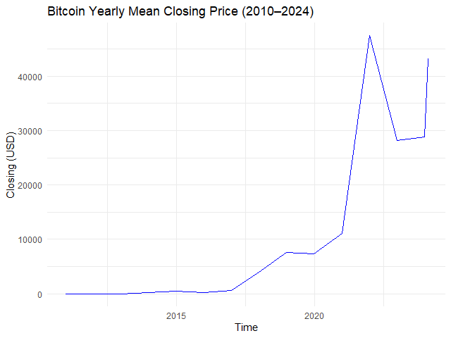
# Example 1. View yearly mean closing price
btc_yr_mean <- apply.yearly(btc_zoo[, "close"],
                            FUN = mean)

# Plot the results
autoplot.zoo(btc_yr_mean) +  
  
  ## Adjust line colour
  geom_line(color = "blue") +
  
  ## Add title and labels
  labs(title = "Bitcoin Yearly Mean Closing Price (2010–2024)",
       x = "Time",
       y = "Closing (USD)") +
  
  ## Use minimal theme
  theme_minimal()

ผลลัพธ์:

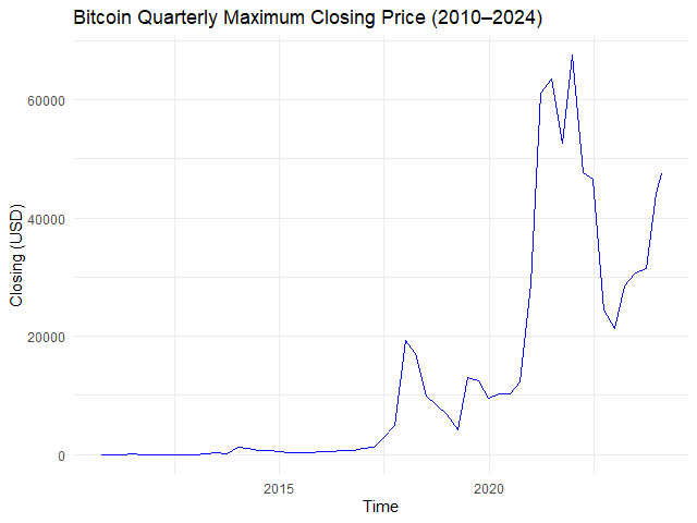
หรือหาราคาปิดสูงสุดในแต่ละไตรมาส:

# Example 2. View quarterly max closing price
btc_qtr_max <- apply.quarterly(btc_zoo[, "close"],
                               FUN = max)

# Plot the results
autoplot.zoo(btc_qtr_max) +  
  
  ## Adjust line colour
  geom_line(color = "blue") +
  
  ## Add title and labels
  labs(title = "Bitcoin Quarterly Maximum Closing Price (2010–2024)",
       x = "Time",
       y = "Closing (USD)") +
  
  ## Use minimal theme
  theme_minimal()

ผลลัพธ์:

ทั้งนี้ ถ้าเราต้องการกำหนดความถี่ของเวลาเอง เราสามารถใช้ endpoints() คู่กับ period.apply() ได้

โดย endpoints() ต้องการ input 3 อย่าง:

x: time series data
on: ระดับช่วงเวลา (เช่น ปี, เดือน, สัปดาห์)
k: จำนวน

และ period.apply() ต้องการ input 3 อย่าง คือ:

x: time series data
INDEX: variable ที่เก็บ endpoints() เอาไว้
FUN: function ที่ใช้สรุปข้อมูล (เช่น mean())

ยกตัวอย่างเช่น เราต้องการหาค่าเฉลี่ยราคาปิด Bitcoin ทุก ๆ 3 เดือน เราจะเขียนภาษา R ได้แบบนี้:

# Create 3-month interval
three_month_eps <- endpoints(x = btc_zoo,
                             on = "months",
                             k = 3)

# Apply the interval
btc_three_month_data <- period.apply(x = btc_zoo[, "close"],
                                     INDEX = three_month_eps,
                                     FUN = mean)

# Plot the results
autoplot.zoo(btc_three_month_data) +  
  
  ## Adjust line colour
  geom_line(color = "blue") +
  
  ## Add title and labels
  labs(title = "Bitcoin 3-Month Average Closing Price (2010–2024)",
       x = "Date",
       y = "Closing Price (USD)") +
  
  ## Use minimal theme
  theme_minimal()

ผลลัพธ์:

🪟 Rolling Window

Rolling window (moving window หรือ sliding window) คือ การสรุปข้อมูลตามช่วงเวลาที่กำหนด โดยช่วงเวลาในการคำนวณจะเคลื่อนตัวไปเรื่อย ๆ

เช่น เราต้องการหาค่าเฉลี่ยของราคาปิด Bitcoin ในช่วง 7 วันล่าสุด การใช้ rolling window จะทำให้เราได้ข้อมูลดังนี้:

Date	Average
2024-01-07	ค่าเฉลี่ยระหว่างวันที่ 1 ถึง 7
2024-01-08	ค่าเฉลี่ยระหว่างวันที่ 2 ถึง 8
2024-01-09	ค่าเฉลี่ยระหว่างวันที่ 3 ถึง 9

ในภาษา R เราสามารถสร้าง rolling window ได้ 2 วิธี:

ใช้ roll*()
ใช้ rollapply()

**1️⃣ roll*()**

เราสามารถสร้าง rolling window ได้ด้วย roll*() จาก zoo package เช่น:

Function	Description
`rollmean()`	หาค่าเฉลี่ย
`rollmedian()`	หาค่ากลาง
`rollmax()`	หาค่าสูงสุด
`rollsum()`	หาผลรวม

roll*() ต้องการ input 3 อย่าง ได้แก่:

x: time series data
k: ช่วงเวลา (window)
align: กำหนดว่า ค่าสรุปที่ได้จะอยู่ด้วยซ้าย ขวา หรือกลางช่วงเวลา
fill: จะแทนค่า missing values หรือไม่

ยกตัวอย่างเช่น เราต้องการหาค่าเฉลี่ยราคาปิด Bitcoin ในช่วง 30 วัน เราจะใช้ rollmean() แบบนี้:

# Create the window for mean price
btc_30_days_roll_mean <- rollmean(x = btc_zoo,
                                  k = 30,
                                  align = "right",
                                  fill = NA)

# Plot the results
autoplot.zoo(btc_30_days_roll_mean[, "close"]) +  
  
  ## Adjust line colour
  geom_line(color = "blue") +
  
  ## Add title and labels
  labs(title = "Bitcoin 30-Day Rolling Mean Price (2010–2024)",
       x = "Time",
       y = "Closing (USD)") +
  
  ## Use minimal theme
  theme_minimal()

ผลลัพธ์:

2️⃣ rollapply()

ในกรณีที่เราต้องการกำหนดการสรุปข้อมูลใน rolling window (เช่น หาค่าต่ำสุด ซึ่งไม่มีใน zoo package) เราสามารถทำได้ด้วย rollapply() ซึ่งต้องการ input 4 อย่างดังนี้:

data: time series data
width: ช่วงเวลา (window)
FUN: การสรุปข้อมูล (เช่น min)
align: กำหนดว่า ค่าสรุปที่ได้จะอยู่ด้วยซ้าย ขวา หรือกลางช่วงเวลา
fill: จะแทนค่า missing values หรือไม่

ยกตัวอย่างเช่น หาราคาปิดต่ำสุดของทุก ๆ 30 วัน:

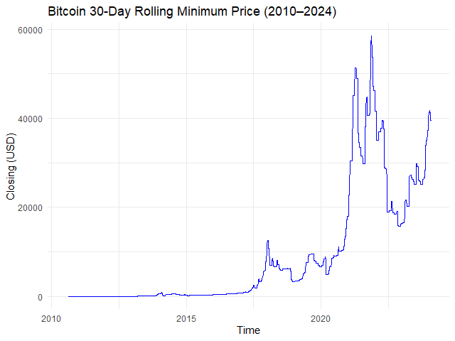
# Creating a rolling window with min() function
btc_30_days_roll_min <- rollapply(data = btc_zoo,
                                  width = 30,
                                  FUN = min,
                                  align = "right",
                                  fill = NA)

# Plot the results
autoplot.zoo(btc_30_days_roll_min[, "close"]) +  
  
  ## Adjust line colour
  geom_line(color = "blue") +
  
  ## Add title and labels
  labs(title = "Bitcoin 30-Day Rolling Minimum Price (2010–2024)",
       x = "Time",
       y = "Closing (USD)") +
  
  ## Use minimal theme
  theme_minimal()

ผลลัพธ์:

➡️ Expanding Window

Expanding window เป็นการสรุปข้อมูลแบบสะสม เช่น:

Date	Average
2024-01-01	หาค่าเฉลี่ยของวันที่ 1
2024-01-02	หาค่าเฉลี่ยของวันที่ 1 + 2
2024-01-03	หาค่าเฉลี่ยของวันที่ 1 + 2 + 3
2024-01-04	หาค่าเฉลี่ยของวันที่ 1 + 2 + 3 + 4
2024-01-05	หาค่าเฉลี่ยของวันที่ 1 + 2 + 3 + 4 + 5

ในภาษา R เราสามารถสร้าง expanding window ได้ด้วย rollapply() โดยเราต้องกำหนดให้:

width เป็นชุดตัวเลข (เช่น 1, 2, 3, …)
align = "right" เสมอ

ยกตัวอย่างเช่น สร้าง expanding window แบบค่าเฉลี่ยราคาปิดของเดือนมกราคม 2024:

# Subset for Jan 2024 data
btc_jan_2024 <- window(x = btc_zoo,
                       start = as.Date("2024-01-01"),
                       end = as.Date("2024-01-31"))

# Create a sequence of widths
btc_jan_2024_width <- seq_along(btc_jan_2024)

# Create an expanding window for mean price
btc_exp_mean <- rollapply(data = btc_2024,
                          width = btc_jan_2024_width,
                          FUN = mean,
                          align = "right",
                          fill = NA)

# Plot the results
autoplot.zoo(btc_exp_mean[, "close"]) +  
  
  ## Adjust line colour
  geom_line(color = "blue") +
  
  ## Add title and labels
  labs(title = "Bitcoin Expanding Mean Price (Jan 2024)",
       x = "Time",
       y = "Closing (USD)") +
  
  ## Use minimal theme
  theme_minimal()

ผลลัพธ์:

😎 Summary

ในบทความนี้ เราได้ทำความรู้จักกับ 7 วิธีการทำงานกับ time series ในภาษา R โดยใช้ base R, lubridate, และ zoo package กัน:

วิธีการทำงาน 1. Converting:

Function	For
`as.Date()`	แปลง character เป็น Date
`as_date()`	แปลง character เป็น Date
`zoo()`	แปลง data frame เป็น `zoo`

วิธีการทำงาน #2. Missing values:

Function	For
`na.fill()`	แทนค่า missing values ด้วยค่าที่กำหนด
`na.locf()`	แทนค่า missing values ตามค่าของข้อมูลที่มาก่อนหน้า
`na.approx()`	แทนค่า missing values ด้วยการวิเคราะห์ข้อมูลที่มาก่อนและหลัง missing values

วิธีการทำงาน #3. Plotting:

Function	For
`autoplot.zoo()`	สร้างกราฟจาก `zoo`

วิธีการทำงาน #4. Subsetting:

Function	For
`window()`	ดึงข้อมูลช่วงเวลาที่ต้องการ
`btc_zoo[boolean_mask, ]`	ดึงข้อมูลช่วงเวลาที่ต้องการ
`btx_zoo[x, y]`	ดึงข้อมูลวันที่ต้องการ

วิธีการทำงาน #5. Aggregating:

Function	For
`apply.daily()`	สรุปข้อมูลรายวัน
`apply.weekly()`	สรุปข้อมูลรายสัปดาห์
`apply.quarterly()`	สรุปข้อมูลรายไตรมาส
`apply.yearly()`	สรุปข้อมูลรายปี
`endpoints()` และ `period.apply()`	สรุปข้อมูลตามช่วงเวลาที่กำหนดเอง

วิธีการทำงาน #6. Rolling window:

Function	For
`rollmean()`	rolling window แบบหาค่าเฉลี่ย
`rollmedian()`	rolling window แบบหาค่ากลาง
`rollmax()`	rolling window แบบหาค่าสูงสุด
`rollsum()`	rolling window แบบหาผลรวม
`rollapply()`	rolling window แบบกำหนดการสรุปข้อมูลเอง

วิธีการทำงาน #7. Expanding window:

Function	For
`seq_along()` และ `rollapply()`	สร้าง expanding window

😺 View Code in GitHub

ดู code และ dataset ในบทความนี้ได้ที่ GitHub

📃 References

✅ R Book for Psychologists: หนังสือภาษา R สำหรับนักจิตวิทยา

📕 ขอฝากหนังสือเล่มแรกในชีวิตด้วยนะครับ 😆

Correlation
t-tests
ANOVA
Reliability
Factor analysis

แล้วทุกคนจะแปลกใจว่า ทำไมภาษา R ง่ายขนาดนี้ 🙂‍↕️

👉 สนใจดูรายละเอียดหนังสือได้ที่ meb:

ดูรายละเอียดหนังสือ R Book for Psychologists

2025-07-17

สอนปลูกต้นไม้ในภาษา R (ภาค 3): 5 ขั้นตอนการสร้าง Boosted Trees ด้วย xgboost package ในภาษา R — ตัวอย่างการทำนายระดับการกินน้ำมันของรถใน mpg dataset
ในบทความนี้ เราจะไปทำความรู้จักกับ eXtreme Gradient Boosting (XGBoost) และวิธีสร้าง XGBoost model ในภาษา R ด้วย xgboost package กัน

ถ้าพร้อมแล้ว ไปเริ่มกันเลย
อ่านเกี่ยวกับการปลูกต้นไม้ในภาษา R ภาคก่อน ๆ ได้ที่:
- ภาค 1: ปลูกด้วย rpart และ randomForest packages
- ภาค 2: ปลูกด้วย ranger package
🚀 XGBoost คืออะไร?

XGBoost เป็น machine learning model ที่จัดอยู่ในกลุ่ม tree-based models หรือ models ที่ทำนายข้อมูลด้วย decision tree อย่าง single decision tree และ random forest

ใน XGBoost, decision trees จะถูกสร้างขึ้นมาเป็นรอบ ๆ โดยในแต่ละรอบ decision trees ใหม่จะเรียนรู้จากความผิดพลาดของรอบก่อน ซึ่งจะทำให้ decision trees ใหม่มีความสามารถที่ดีขึ้นเรื่อย ๆ

เมื่อสิ้นสุดการสร้าง XGBoost ใช้ผลรวมของ decision trees ทุกต้นในการทำนายข้อมูล ดังนี้:
- Regression problem: หาค่าเฉลี่ยแบบถ่วงน้ำหนักจากทุกต้น
- Classification problem: ทำนายผลลัพธ์ด้วยค่าเฉลี่ยความน่าจะเป็นจากทุกต้น
💻 XGBoost ในภาษา R

ในภาษา R เราสามารถสร้าง XGBoost ได้ด้วย xgboost package ใน 5 ขั้นตอน ได้แก่:
1. Install and load the package
2. Load and prepare the data
3. Split the data
4. Train the model
5. Evaluate the model
1️⃣ Install & Load the Package

ในขั้นแรก ให้เราติดตั้งและเรียกใช้งาน xgboost package

ติดตั้ง:
```
# Install
install.packages("xgboost")
```
เรียกใช้งาน:
```
# Load
library(xgboost)
```
2️⃣ Load & Prepare the Data

ในขั้นตอนที่สอง ให้เราโหลดและเตรียมข้อมูลที่จะใช้สร้าง XGBoost model โดยในบทความนี้ เราจะใช้ mpg dataset จาก ggplot2 package กัน

mpg ประกอบด้วยข้อมูลรถและระดับการใช้น้ำมัน และจุดประสงค์ของเรา คือ ทำนายระดับการกินน้ำมันเมื่อรถวิ่งบน highway (hwy)

เราสามารถโหลด mpg ได้ผ่าน ggplot2:
```
# Install ggplot2
install.packages("ggplot2")

# Load ggplot2
library(ggplot2)

# Load the dataset
data(mpg)
```
เมื่อโหลด dataset แล้ว เราสามารถสำรวจข้อมูลได้ด้วย head():
```
# Preview
head(mpg)
```
ผลลัพธ์:
```
# A tibble: 6 × 11
  manufacturer model displ  year   cyl trans      drv     cty   hwy fl    class  
  <chr>        <chr> <dbl> <int> <int> <chr>      <chr> <int> <int> <chr> <chr>  
1 audi         a4      1.8  1999     4 auto(l5)   f        18    29 p     compact
2 audi         a4      1.8  1999     4 manual(m5) f        21    29 p     compact
3 audi         a4      2    2008     4 manual(m6) f        20    31 p     compact
4 audi         a4      2    2008     4 auto(av)   f        21    30 p     compact
5 audi         a4      2.8  1999     6 auto(l5)   f        16    26 p     compact
6 audi         a4      2.8  1999     6 manual(m5) f        18    26 p     compact
```
และดูโครงสร้างข้อมูลด้วย str():
```
# View the tructure
str(mpg)
```
ผลลัพธ์:
```
tibble [234 × 11] (S3: tbl_df/tbl/data.frame)
 $ manufacturer: chr [1:234] "audi" "audi" "audi" "audi" ...
 $ model       : chr [1:234] "a4" "a4" "a4" "a4" ...
 $ displ       : num [1:234] 1.8 1.8 2 2 2.8 2.8 3.1 1.8 1.8 2 ...
 $ year        : int [1:234] 1999 1999 2008 2008 1999 1999 2008 1999 1999 2008 ...
 $ cyl         : int [1:234] 4 4 4 4 6 6 6 4 4 4 ...
 $ trans       : chr [1:234] "auto(l5)" "manual(m5)" "manual(m6)" "auto(av)" ...
 $ drv         : chr [1:234] "f" "f" "f" "f" ...
 $ cty         : int [1:234] 18 21 20 21 16 18 18 18 16 20 ...
 $ hwy         : int [1:234] 29 29 31 30 26 26 27 26 25 28 ...
 $ fl          : chr [1:234] "p" "p" "p" "p" ...
 $ class       : chr [1:234] "compact" "compact" "compact" "compact" ...
```
จากผลลัพธ์ เราจะเห็นได้ว่า mpg มี columns ที่เราต้องปรับจาก character เป็น factor อยู่ เช่น manufacturer, model ซึ่งเราสามารถปรับได้ดังนี้:
```
# Convert character columns to factor

## Get character columns
chr_cols <- c("manufacturer",
              "model",
              "trans",
              "drv",
              "fl",
              "class")

## For-loop through the character columns
for (col in chr_cols) {
  mpg[[col]] <- as.factor(mpg[[col]])
}

## Check the results
str(mpg)
```
ผลลัพธ์:
```
tibble [234 × 11] (S3: tbl_df/tbl/data.frame)
 $ manufacturer: Factor w/ 15 levels "audi","chevrolet",..: 1 1 1 1 1 1 1 1 1 1 ...
 $ model       : Factor w/ 38 levels "4runner 4wd",..: 2 2 2 2 2 2 2 3 3 3 ...
 $ displ       : num [1:234] 1.8 1.8 2 2 2.8 2.8 3.1 1.8 1.8 2 ...
 $ year        : int [1:234] 1999 1999 2008 2008 1999 1999 2008 1999 1999 2008 ...
 $ cyl         : int [1:234] 4 4 4 4 6 6 6 4 4 4 ...
 $ trans       : Factor w/ 10 levels "auto(av)","auto(l3)",..: 4 9 10 1 4 9 1 9 4 10 ...
 $ drv         : Factor w/ 3 levels "4","f","r": 2 2 2 2 2 2 2 1 1 1 ...
 $ cty         : int [1:234] 18 21 20 21 16 18 18 18 16 20 ...
 $ hwy         : int [1:234] 29 29 31 30 26 26 27 26 25 28 ...
 $ fl          : Factor w/ 5 levels "c","d","e","p",..: 4 4 4 4 4 4 4 4 4 4 ...
 $ class       : Factor w/ 7 levels "2seater","compact",..: 2 2 2 2 2 2 2 2 2 2 ...
```
ตอนนี้ columns ที่เราต้องการถูกเปลี่ยนเป็น factor เรียบร้อยแล้ว

3️⃣ Split the Data

ในขั้นที่สาม เราจะทำ 3 อย่างด้วยกัน คือ:
1. แยกตัวแปรต้น (x) และตัวแปรตาม (y) ออกจากกัน
2. แบ่งข้อมูลออกเป็น training และ test sets
3. แปลงข้อมูลให้เป็น DMatrix
ข้อที่ 1. เราสามารถแยกตัวแปรต้นและตัวแปรตามออกจากกันได้ดังนี้:
```
# Separate the features from the outcome

## Get the features
x <- mpg[, !names(mpg) %in% "hwy"]

## One-hot encode the features
x <- model.matrix(~ . - 1,
                  data = x)

## Get the outcome
y <- mpg$hwy
```
สังเกตว่า ตอนที่เราแยกตัวแปรต้น เราแปลงตัวแปรเหล่านี้เป็น 0, 1 ด้วย one-hot encoding ด้วย เนื่องจาก xgboost ต้องการตัวแปรต้นที่เป็น numeric

.

ข้อที่ 2. จากนั้น เราจะแบ่ง dataset เป็น training (80%) และ test sets (20%) ดังนี้:
```
# Split the data

## Set seed for reproducibility
set.seed(360)

## Get training index
train_index <- sample(1:nrow(x),
                      nrow(x) * 0.8)

## Create x, y train
x_train <- x[train_index, ]
y_train <- y[train_index]

## Create x, y test
x_test <- x[-train_index, ]
y_test <- y[-train_index]

## Check the results
cat("TRAIN SET", "\\n")
cat("1. Data in x_train:", nrow(x_train), "\\n")
cat("2. Data in y_train:", length(y_train), "\\n")
cat("---", "\\n", "TEST SET", "\\n")
cat("1. Data in x_test:", nrow(x_test), "\\n")
cat("2. Data in y_test:", length(y_test), "\\n")
```
ผลลัพธ์:
```
TRAIN SET
1. Data in x_train: 187
2. Data in y_train: 187
---
TEST SET
1. Data in x_test: 47
2. Data in y_test: 47
```
.

ข้อที่ 3. สุดท้าย เราจะแปลง x, y เป็น DMatrix ซึ่งเป็น object ที่ xgboost ใช้ในการสร้าง XGboost model ดังนี้:
```
# Convert to DMatrix

## Training set
train_set <- xgb.DMatrix(data = x_train,
                         label = y_train)

## Test set
test_set <- xgb.DMatrix(data = x_test,
                        label = y_test)

## Check the results
train_set
test_set
```
ผลลัพธ์:
```
TRAIN SET
xgb.DMatrix  dim: 187 x 77  info: label  colnames: yes
---
TEST SET
xgb.DMatrix  dim: 47 x 77  info: label  colnames: yes
```
4️⃣ Train the Model

ในขั้นที่สี่ เราจะสร้าง XGBoost model ด้วย xgb.train() ซึ่งต้องการ 5 arguments ดังนี้:
xgb.train(params, data, nrounds, watchlist, verbose)
1. params = hyperparametre ที่ต้องการใช้สร้าง model ที่ดีที่สุด
2. data = training set ที่ใช้สร้าง model
3. nrounds = จำนวนครั้งในการในสร้าง decision trees
4. watchlist = ชุดข้อมูลที่ต้องการใช้ประเมินความสามารถของ model
5. verbose = พิมพ์ข้อมูลในระหว่างการสร้าง model (1) หรือไม่ (0)
(Note: ศึกษา argument อื่น ๆ ของ xgb.train() ได้ที่ XGBoost Parameters)

สำหรับบทความนี้ เราจะใช้ xgb.train() ดังนี้:
```
# Train the model

## Set hyperparametres
hp <- list(objective = "reg:squarederror",
           eta = 0.1,
           max_depth = 4,
           eval_metric = c("rmse",
                           "mae"))

## Train
xgb_model <- xgb.train(params = hp,
                       data = train_set,
                       nrounds = 50,
                       watchlist = list(train = train_set,
                                        test = test_set),
                       verbose = 1)
```
ผลลัพธ์:
```
[1]	train-rmse:21.083975	test-rmse:22.739357 
[2]	train-rmse:19.045063	test-rmse:20.598582 
[3]	train-rmse:17.204130	test-rmse:18.713079 
[4]	train-rmse:15.549113	test-rmse:16.974701 
[5]	train-rmse:14.053049	test-rmse:15.453560 
[6]	train-rmse:12.707307	test-rmse:14.097377 
[7]	train-rmse:11.495216	test-rmse:12.877722 
[8]	train-rmse:10.402476	test-rmse:11.767320 
[9]	train-rmse:9.413522	test-rmse:10.740546 
[10]	train-rmse:8.525230	test-rmse:9.863130 
[11]	train-rmse:7.722776	test-rmse:9.068840 
[12]	train-rmse:7.000648	test-rmse:8.357181 
[13]	train-rmse:6.346603	test-rmse:7.687483 
[14]	train-rmse:5.758685	test-rmse:7.091249 
[15]	train-rmse:5.229548	test-rmse:6.557082 
[16]	train-rmse:4.753713	test-rmse:6.079389 
[17]	train-rmse:4.325653	test-rmse:5.651858 
[18]	train-rmse:3.940325	test-rmse:5.275154 
[19]	train-rmse:3.594545	test-rmse:4.938849 
[20]	train-rmse:3.283961	test-rmse:4.627743 
[21]	train-rmse:3.003089	test-rmse:4.352060 
[22]	train-rmse:2.747553	test-rmse:4.110172 
[23]	train-rmse:2.519617	test-rmse:3.889650 
[24]	train-rmse:2.314957	test-rmse:3.691806 
[25]	train-rmse:2.133630	test-rmse:3.499208 
[26]	train-rmse:1.969083	test-rmse:3.330280 
[27]	train-rmse:1.823011	test-rmse:3.181541 
[28]	train-rmse:1.693565	test-rmse:3.045308 
[29]	train-rmse:1.575817	test-rmse:2.919070 
[30]	train-rmse:1.469256	test-rmse:2.812063 
[31]	train-rmse:1.375599	test-rmse:2.700515 
[32]	train-rmse:1.292928	test-rmse:2.615973 
[33]	train-rmse:1.218867	test-rmse:2.541929 
[34]	train-rmse:1.151134	test-rmse:2.462113 
[35]	train-rmse:1.092395	test-rmse:2.404873 
[36]	train-rmse:1.039158	test-rmse:2.336600 
[37]	train-rmse:0.993882	test-rmse:2.291398 
[38]	train-rmse:0.952062	test-rmse:2.236936 
[39]	train-rmse:0.915935	test-rmse:2.198657 
[40]	train-rmse:0.879957	test-rmse:2.152984 
[41]	train-rmse:0.850423	test-rmse:2.102272 
[42]	train-rmse:0.822475	test-rmse:2.054172 
[43]	train-rmse:0.799025	test-rmse:2.011621 
[44]	train-rmse:0.775398	test-rmse:1.971787 
[45]	train-rmse:0.755066	test-rmse:1.933539 
[46]	train-rmse:0.736655	test-rmse:1.900084 
[47]	train-rmse:0.719087	test-rmse:1.870832 
[48]	train-rmse:0.705279	test-rmse:1.853400 
[49]	train-rmse:0.691914	test-rmse:1.834918 
[50]	train-rmse:0.680016	test-rmse:1.825738 
```
จะเห็นได้ว่า model ในแต่ละรอบมี RMSE หรือตัวบ่งชี้ความคลาดเคลื่อน ที่ลดลงเรื่อย ๆ เนื่องจาก model ใหม่เรียนรู้จากความผิดพลาดของ model ก่อนหน้า

หลังจากสร้าง model เสร็จแล้ว เราสามารถดูรายละเอียดของ model ได้แบบนี้:
```
# Print the model
xgb_model
```
ผลลัพธ์:
```
##### xgb.Booster
raw: 62.4 Kb 
call:
  xgb.train(params = hp, data = train_set, nrounds = 50, watchlist = list(train = train_set, 
    test = test_set), verbose = 1)
params (as set within xgb.train):
  objective = "reg:squarederror", eta = "0.1", max_depth = "4", eval_metric = "rmse", validate_parameters = "mae", objective = "TRUE"
xgb.attributes:
  niter
callbacks:
  cb.print.evaluation(period = print_every_n)
  cb.evaluation.log()
# of features: 77 
niter: 50
nfeatures : 77 
evaluation_log:
  iter train_rmse test_rmse
 <num>      <num>     <num>
     1 21.0839746 22.739357
     2 19.0450628 20.598582
   ---        ---       ---
    49  0.6919137  1.834918
    50  0.6800159  1.825738
```
5️⃣ Evaluate the Model

ในขั้นสุดท้าย เราจะประเมินความสามารถของ model ใน 3 ขั้นตอนกัน คือ:
1. ใช้ model ทำนายตัวแปรตาม
2. คำนวณ MAE, RMSE, และ R squared
3. Print MAE, RMSE, และ R squared
.

ข้อที่ 1. ใช้ model ทำนายตัวแปรตาม ด้วย predict():
```
# Make predictions
y_pred <- predict(xgb_model,
                  newdata = x_test)

# Compare predictions to actual outcomes
results <- data.frame(actual = y_test,
                      predicted = y_pred,
                      error = y_test - y_pred)

# Preview the results
head(results, 10)
```
ผลลัพธ์:
```
   actual predicted      error
1      31  27.81219  3.1878090
2      25  25.89449 -0.8944893
3      30  30.13318 -0.1331844
4      29  26.77814  2.2218552
5      24  24.34723 -0.3472347
6      23  23.58175 -0.5817528
7      19  17.81131  1.1886921
8      12  12.32908 -0.3290768
9      12  12.31534 -0.3153391
10     16  16.25793 -0.2579288
```
.

ข้อที่ 2. คำนวณ MAE, RMSE, และ R squared ซึ่งเป็นตัวชี้วัดความสามารถของ regression models:
```
# Calculate MAE
mae <- mean(abs(results$error))

# Calculate RMSE
rmse <- sqrt(mean((results$error)^2))

# Calculate R squared
ss_res <- sum((results$error)^2)
ss_tot <- sum((results$actual - mean(results$actual))^2)
r_squared <- 1 - (ss_res / ss_tot)
```
.

ข้อที่ 3. แสดงผลลัพธ์:
```
# Print the results
cat("MAE:", round(mae, 2), "\\n")
cat("RMSE:", round(rmse, 2), "\\n")
cat("R squared:", round(r_squared, 2), "\\n")
```
ผลลัพธ์:
```
MAE: 1.23
RMSE: 1.83
R squared: 0.93 
```
จะเห็นได้ว่า model ของเราสามารถอธิบายตัวแปรตามได้ถึง 93% (R squared) และมีความคลาดเคลื่อนโดยเฉลี่ย 1.23 miles per gallon (MAE)

💪 Summary

ในบทความนี้ เราได้ไปทำความรู้จักการสร้าง boosted tree ด้วย xgboost package ในภาษา R ซึ่งมีการทำงาน 5 ขั้นตอนกัน:
1. Install and load the package
2. Load and prepare the data
3. Split the data
4. Train the model
5. Evaluate the model
😺 GitHub

ดู code ทั้งหมดในบทความนี้ได้ที่ GitHub

📃 References
✅ R Book for Psychologists: หนังสือภาษา R สำหรับนักจิตวิทยา

📕 ขอฝากหนังสือเล่มแรกในชีวิตด้วยนะครับ 😆

🙋 ใครที่กำลังเรียนจิตวิทยาหรือทำงานสายจิตวิทยา และเบื่อที่ต้องใช้ software ราคาแพงอย่าง SPSS และ Excel เพื่อทำข้อมูล

💪 ผมขอแนะนำ R Book for Psychologists หนังสือสอนใช้ภาษา R เพื่อการวิเคราะห์ข้อมูลทางจิตวิทยา ที่เขียนมาเพื่อนักจิตวิทยาที่ไม่เคยมีประสบการณ์เขียน code มาก่อน

ในหนังสือ เราจะปูพื้นฐานภาษา R และพาไปดูวิธีวิเคราะห์สถิติที่ใช้บ่อยกัน เช่น:
- Correlation
- t-tests
- ANOVA
- Reliability
- Factor analysis
🚀 เมื่ออ่านและทำตามตัวอย่างใน R Book for Psychologists ทุกคนจะไม่ต้องพึง SPSS และ Excel ในการทำงานอีกต่อไป และสามารถวิเคราะห์ข้อมูลด้วยตัวเองได้ด้วยความมั่นใจ

แล้วทุกคนจะแปลกใจว่า ทำไมภาษา R ง่ายขนาดนี้ 🙂‍↕️

👉 สนใจดูรายละเอียดหนังสือได้ที่ meb:

ดูรายละเอียดหนังสือ R Book for Psychologists
Share this:
X
Facebook
Like Loading…
2025-07-03

Generalised Linear Model: วิธีใช้ glm() ในภาษา R เพื่อทำนายข้อมูลที่ไม่ปกติ — Linear, Logistic, และ Poisson Regression

ในบทความนี้ เราจะไปทำความรู้จักกับ generalised linear model (GLM) และวิธีทำ GLM ในภาษา R กัน

ถ้าพร้อมแล้ว ไปเริ่มกันเลย

🤔 GLM คืออะไร?

GLM เป็นเทคนิคทางสถิติที่ใช้ทำนายข้อมูลที่มีการกระจายตัวไม่ปกติ (non-normal distribution) เช่น ข้อมูลที่มีผลลัพธ์เพียง 0 และ 1

GLM ทำนายข้อมูลเหล่านี้โดยการต่อยอดจากสมการเส้นตรง (linear model) และมี 3 องค์ประกอบ ได้แก่:

Family: การกระจายตัวของตัวแปรตาม (y)
Linear predictors: สมการเส้นตัวตรงของตัวแปรต้น (x) หรือตัวแปรทำนาย (predictor)
Link function: function ที่เชื่อมตัวแปรต้นกับตัวแปรตามเข้าด้วยกัน

💻 GLM ในภาษา R

ในภาษา R เราสามารถใช้งาน GLM ได้ผ่าน glm() function ซึ่งต้องการข้อมูล 3 อย่าง:

glm(formula, data, family)

formula = ความสัมพันธ์ระหว่างตัวแปรต้นและตัวแปรตาม ในรูปแบบ y ~ x
data = ชุดข้อมูลที่ใช้ในการวิเคราะห์
family = การกระจายตัวของตัวแปรตาม

จะสังเกตว่า glm() ไม่มี parametre สำหรับ link function ทั้งนี้เป็นเพราะ glm() เรียกใช้ link function ให้อัตโนมัติตาม family ที่เรากำหนด

ทั้งนี้ ประเภทข้อมูล, family, และ link function ที่เราสามารถเรียกใช้ glm() ได้มีดังนี้:

Data	family	Link Function
Normal	`gaussian`	`link = "identity”`
Binomial	`binomial`	`link = "logit”`
Poisson	`poisson`	`link = "log”`
Quasi-poisson	`quasipoisson`	`link = "log”`
Gamma	`Gamma`	`link = "inverse”`

เราไปดูตัวอย่างการใช้งาน glm() เพื่อทำนายและแปลผลกัน

☕ ตัวอย่างข้อมูล: coffee_shop

เราจะไปดูตัวอย่างการใช้ glm() เพื่อทำนายข้อมูล 3 ประเภทกัน:

Linear regression
Logistic regression
Poisson regression

โดยเราจะใช้ตัวอย่างเป็นข้อมูลจำลองชื่อ coffee_shop ซึ่งประกอบด้วยข้อมูลการขายจากร้านกาแฟแห่งหนึ่ง และมีรายละเอียดดังนี้:

No.	Column	Description
1	`day`	วันที่
2	`temp`	อุณหภูมิโดยเฉลี่ยของวัน
3	`promo`	เป็นวันที่มีโปรโมชัน (มี, ไม่มี)
4	`weekend`	เป็นวันหยุดสุดสัปดาห์ (วันหยุด, วันธรรมดา)
5	`sales`	ยอดขาย
6	`customers`	จำนวนลูกค้าในแต่ละวัน
7	`sold_out`	ขายหมด (หมด, ไม่หมด)

ก่อนวิเคราะห์ข้อมูล เราจะสร้าง coffee_shop ตามนี้:

# Generate mock coffee shop dataset (15 days)

## Set seed for reproducibility
set.seed(123)

## Generate
coffee_shop <- data.frame(
  
  ## Generate 15 days
  day = 1:15,
  
  ## Generate daily temperature
  temp = round(rnorm(15,
                     mean = 25,
                     sd = 5),
               1),
  
  ## Generate promotion day
  promo = sample(c(0, 1),
                 15,
                 replace = TRUE),
  
  ## Generate weekend
  weekend = c(0, 0, 0, 0, 1, 1, 0, 0, 0, 1, 1, 0, 0, 0, 1),
  
  ## Generate the number of sales
  sales = round(rnorm(15,
                      mean = 300,
                      sd = 50)),
  
  ## Generate the number of daily customers
  customers = rpois(15,
                    lambda = 80),
  
  ## Generate sold-out
  sold_out = sample(c(0, 1),
                    15,
                    replace = TRUE)
)

## Convert binary variables to factors
coffee_shop$promo <- factor(coffee_shop$promo,
                            levels = c(0, 1),
                            labels = c("NoPromo", "Promo"))

coffee_shop$weekend <- factor(coffee_shop$weekend,
                              levels = c(0, 1),
                              labels = c("Weekday", "Weekend"))

coffee_shop$sold_out <- factor(coffee_shop$sold_out,
                               levels = c(0, 1),
                               labels = c("No", "Yes"))

## View the dataset
print(coffee_shop)

ผลลัพธ์:

   day temp   promo weekend sales customers sold_out
1    1 22.2 NoPromo Weekday   246        73      Yes
2    2 23.8   Promo Weekday   296        76      Yes
3    3 32.8 NoPromo Weekday   354        83       No
4    4 25.4   Promo Weekday   293        87       No
5    5 25.6   Promo Weekend   242        78      Yes
6    6 33.6 NoPromo Weekend   259        91      Yes
7    7 27.3 NoPromo Weekday   334        71      Yes
8    8 18.7 NoPromo Weekday   284        76       No
9    9 21.6 NoPromo Weekday   234        72      Yes
10  10 22.8   Promo Weekend   270        79       No
11  11 31.1 NoPromo Weekend   294        82      Yes
12  12 26.8   Promo Weekday   344        79       No
13  13 27.0   Promo Weekday   292        79       No
14  14 25.6 NoPromo Weekday   316        92       No
15  15 22.2 NoPromo Weekend   139        77      Yes

เราไปดูวิธีทำนายข้อมูลกัน

1️⃣ Linear Regression

Linear regression เป็นการทำนายข้อมูล numeric เช่น ยอดขาย (sales) ซึ่งเราสามารถใช้ glm() ทำนายได้ดังนี้:

# Create a regression model with glm()
linear_reg <- glm(sales ~ temp + promo + weekend,
                  data = coffee_shop,
                  family = gaussian)

เราสามารถดู model ได้ด้วย summary():

# Get model summary
summary(linear_reg)

ผลลัพธ์:

Call:
glm(formula = sales ~ temp + promo + weekend, family = gaussian, 
    data = coffee_shop)

Coefficients:
               Estimate Std. Error t value Pr(>|t|)   
(Intercept)      96.599     59.669   1.619  0.13375   
temp              7.703      2.283   3.373  0.00621 **
promoPromo       23.014     18.537   1.241  0.24025   
weekendWeekend  -73.444     19.654  -3.737  0.00328 **
---
Signif. codes:  0 ‘***’ 0.001 ‘**’ 0.01 ‘*’ 0.05 ‘.’ 0.1 ‘ ’ 1

(Dispersion parameter for gaussian family taken to be 1222.243)

    Null deviance: 39702  on 14  degrees of freedom
Residual deviance: 13445  on 11  degrees of freedom
AIC: 154.54

Number of Fisher Scoring iterations: 2

จากผลลัพธ์ เราจะเห็นความสำคัญของตัวแปรต้นและ coefficient ซึ่งระบุการเปลี่ยนแปลงของตัวแปรตามการเปลี่ยนของตัวแปรต้น:

ตัวแปรที่สามารถทำนาย sales ได้อย่างมีนัยสำคัญ คือ temp และ weekend (สังเกตจาก **)
promo ไม่สามารถทำนาย sales ได้อย่างมีนัยสำคัญ
Coefficient ของ temp คือ 7.70 ซึ่งหมายถึง อุณหภูมิเปลี่ยน 1 หน่วย ยอดขายจะเพิ่มขึ้น 7.70 หน่วย
Coefficient ของ weekend คือ -73.44 ซึ่งหมายถึง วันหยุดสุดสัปดาห์ ยอดขายจะลดลง 73.44 หน่วย

2️⃣ Logistic Regression

Logistic regression เป็นการทำนายข้อมูลที่เป็นมีผลลัพธ์เพียง 2 ค่า เช่น:

ใช่, ไม่ใช่
ผ่าน, ไม่ผ่าน
ตรง, ไม่ตรง

ใน coffee_shop เรามี sold_out ซึ่งเราสามารถทำนายด้วย logistic regression ด้วย glm() ได้แบบนี้:

# Create a logistic regression model
log_reg <- glm(sold_out ~ temp + promo + weekend,
               data = coffee_shop,
               family = binomial)

จากนั้น ดู model ด้วย summary():

# Get model summary
summary(log_reg)

ผลลัพธ์:

Call:
glm(formula = sold_out ~ temp + promo + weekend, family = binomial, 
    data = coffee_shop)

Coefficients:
               Estimate Std. Error z value Pr(>|z|)
(Intercept)     1.30934    3.92442   0.334    0.739
temp           -0.04448    0.15189  -0.293    0.770
promoPromo     -1.73681    1.31881  -1.317    0.188
weekendWeekend  2.15038    1.45643   1.476    0.140

(Dispersion parameter for binomial family taken to be 1)

    Null deviance: 20.728  on 14  degrees of freedom
Residual deviance: 16.426  on 11  degrees of freedom
AIC: 24.426

Number of Fisher Scoring iterations: 4

จะเห็นได้ว่า หน้าตาผลลัพธ์คล้ายกับ linear regression แต่สิ่งที่แตกต่างกัน คือ coefficient อยู่ในรูป log-odd ซึ่งเราสามารถถอดรูปได้ด้วย exp() เพื่อแปลผล:

# Transform coefficient
exp(coef(log_reg))

ผลลัพธ์:

   (Intercept)           temp     promoPromo weekendWeekend 
     3.7037124      0.9564938      0.1760812      8.5881237

เราสามารถแปลผลได้ดังนี้:

Predictor	Coefficient	Interpretation
`temp`	0.96	เมื่ออุณหภูมิสูงขึ้น 1 หน่วย ร้านมีโอกาสขายหมดเพิ่มขึ้น 0.96
`promo`	0.18	เมื่อมีโปรโมชัน ร้านมีโอกาสขายหมดเพิ่มขึ้น 0.18
`weekend`	8.59	เมื่อเป็นวันสุดสัปดาห์ ร้านมีโอกาสขายหมดเพิ่มขึ้น 8.59

3️⃣ Poisson Regression

Poisson regression เป็นการทำนายข้อมูลการนับ (count data) หรือข้อมูลที่เกิดขึ้นในช่วงเวลาที่กำหนด เช่น:

จำนวนรถบนถนนในแต่ละชั่วโมง
จำนวนข้อความที่ได้รับใน 1 วัน
จำนวนสินค้าที่ขายได้ใน 3 เดือน

ใน coffee_shop เรามี customers ซึ่งสามารถทำนาย poisson regression ผ่าน glm() ได้ดังนี้:

# Create a poisson regression model
poisson_reg <- glm(customers ~ temp + promo + weekend,
                   data = coffee_shop,
                   family = poisson)

ดู model:

# Get model summary
summary(poisson_reg)

ผลลัพธ์:

Call:
glm(formula = customers ~ temp + promo + weekend, family = poisson, 
    data = coffee_shop)

Coefficients:
               Estimate Std. Error z value Pr(>|z|)    
(Intercept)    4.108939   0.192499  21.345   <2e-16 ***
temp           0.010077   0.007299   1.381    0.167    
promoPromo     0.010327   0.059616   0.173    0.862    
weekendWeekend 0.012692   0.062739   0.202    0.840    
---
Signif. codes:  0 ‘***’ 0.001 ‘**’ 0.01 ‘*’ 0.05 ‘.’ 0.1 ‘ ’ 1

(Dispersion parameter for poisson family taken to be 1)

    Null deviance: 7.0199  on 14  degrees of freedom
Residual deviance: 4.8335  on 11  degrees of freedom
AIC: 106.06

Number of Fisher Scoring iterations: 3

Coefficient ของ poisson regression อยู่ในรูป log เช่นเดียวกับ logistic regression ดังนั้น เราจะถอดรูปด้วย exp() ก่อนแปลผล:

# Transform the coefficients
exp(coef(poisson_reg))

ผลลัพธ์:

   (Intercept)           temp     promoPromo weekendWeekend 
     60.882073       1.010127       1.010381       1.012773

จะเห็นได้ว่า coefficient ของทั้ง 3 ตัวแปรต้นอยู่ที่ 1.01 ซึ่งหมายถึง การเปลี่ยนแปลงตัวแปรต้นตัวใดตัวหนึ่ง ทำให้จำนวนลูกค้าเพิ่มขึ้น 1 คน

💪 Summary

ในบทความนี้ เราได้ไปทำความรู้จักกับ GLM ซึ่งเป็นเทคนิคทางสถิติที่ใช้ทำนายข้อมูลที่ไม่ปกติ และได้ดูวิธีการใช้ glm() function ในภาษา R เพื่อทำนายข้อมูล 3 ประเภท:

Linear regression
Logistic regression
Poisson regression

😺 GitHub

ดู code ทั้งหมดในบทความนี้ได้ที่ GitHub

📃 References

What is GLM?

GLM in R:

✅ R Book for Psychologists: หนังสือภาษา R สำหรับนักจิตวิทยา

📕 ขอฝากหนังสือเล่มแรกในชีวิตด้วยนะครับ 😆

Correlation
t-tests
ANOVA
Reliability
Factor analysis

แล้วทุกคนจะแปลกใจว่า ทำไมภาษา R ง่ายขนาดนี้ 🙂‍↕️

👉 สนใจดูรายละเอียดหนังสือได้ที่ meb:

ดูรายละเอียดหนังสือ R Book for Psychologists

2025-06-26

tidymodels: แนะนำวิธีใช้แพ็กเกจ machine learning ที่ทรงพลัง ครบจบ และทันสมัยในภาษา R เพื่อสร้าง ประเมิน และปรับทูน model — ตัวอย่างการทำนายราคาบ้านใน Boston dataset

ในการทำ machine learning (ML) ในภาษา R เรามี packages และ functions ที่หลากหลายให้เลือกใช้งาน ซึ่งแต่ละ package และ function มีวิธีใช้งานที่แตกต่างกันไป

ยกตัวอย่างเช่น:

glm() จาก base R สำหรับสร้าง regression models ต้องการ input 3 อย่าง คือ formula, data, และ family:

glm(formula, data, family)

knn() จาก class package สำหรับสร้าง KNN model ต้องการ input 4 อย่าง คือ ตัวแปรต้นของ training set, ตัวแปรต้นของ test set, ตัวแปรตามของ training set, และค่า k:

knn(train_x, test_x, train_y, k)

rpart() จาก rpart package สำหรับสร้าง decision tree model ต้องการ input 2 อย่าง คือ formula และ data:

rpart(formula, data)

…

การใช้งาน function ที่แตกต่างกันทำให้การสร้าง ML models เกิดความซับซ้อนโดยไม่จำเป็น และทำให้เกิดความผิดพลาดในการทำงานได้ง่าย

tidymodels เป็น package ที่ถูกออกแบบมาเพื่อแก้ปัญหานี้โดยเฉพาะ

tidymodels เป็น meta-package หรือ package ที่รวบรวม packages อื่นเอาไว้ เมื่อเราโหลด tidymodels เราจะสามารถใช้งาน 8 packages ที่ออกแบบมาให้ทำงานร่วมกัน ช่วยให้เราทำงาน ML ได้ครบ loop

ทั้ง 8 packages ใน tidymodels ได้แก่:

No.	Package	ML Phase	For
1	`rsample`	Pre-processing	Data resampling
2	`recipes`	Pre-processing	Feature engineering
3	`parsnip`	Modelling	Model fitting
4	`tune`	Post-processing	Hyperparameter tuning
5	`dials`	Post-processing	Hyperparameter tuning
6	`yardstick`	Post-processing	Model evaluation
7	`broom`	Post-processing	Format ผลลัพธ์ให้ดูง่าย
8	`workflow`	All	รวม pre-processing, modeling, and post-processing ให้เป็น pipeline เดียวกัน

ในบทความนี้ เราจะมาดูวิธีใช้ tidymodels เพื่อสร้าง ML models กัน

ถ้าพร้อมแล้ว ไปเริ่มกันเลย

🔢 Dataset

🏠 Boston

ในบทความนี้ เราจะใช้ Boston dataset จาก MASS package เป็นตัวอย่างในการทำงานกับ tidymodels กัน

Boston เป็นชุดข้อมูลบ้านในเมืองบอสตัน รัฐแมสซาชูเซส ประเทศอเมริกา และมีข้อมูลทั้งหมด 14 columns ดังนี้:

No.	Column	Description
1	`crim`	ระดับอาชญากรรมในแต่ละเขต
2	`zn`	สัดส่วนพื้นที่อาศัย
3	`indus`	สัดส่วนธุรกิจที่เป็น non-retail ในแต่ละเขต
4	`chas`	เป็นพื้นที่ติดกับ Charles River ไหม (1 = ติด, 0 = ไม่ติด)
5	`nox`	ระดับ nitrogen oxide
6	`rm`	จำนวนห้องโดยเฉลี่ย
7	`age`	สัดส่วย unit ที่มีคนเข้าอยู่ ซึ่งถูกสร้างก่อนปี ค.ศ. 1940
8	`dis`	ระยะทางจากพื้นที่ทำงานในเมืองบอสตัน
9	`rad`	ระดับการเข้าถึง radial highways
10	`tax`	ภาษีโรงเรือน
11	`ptratio`	สัดส่วนนักเรียนต่อครูในแต่ละเขต
12	`black`	สัดส่วนผู้อยู่อาศัยที่เป็นคนผิวดำ
13	`lstat`	สัดส่วนของประชากรที่มีฐานะยากจน
14	`medv`	ราคากลางของบ้านที่มีผู้อยู่อาศัย

Note: อ่านรายละเอียดเพิ่มเติมเกี่ยวกับ Boston dataset ได้ที่ A Complete Guide to the Boston Dataset in R

จุดประสงค์ของเราในการทำงานกับ Boston dataset คือ ทำนายราคาบ้าน (medv)

⬇️ Get Boston

ในการใช้งาน Boston เราสามารถเรียกใช้งานได้ผ่าน MASS package ดังนี้:

ติดตั้ง MASS package
โหลด MASS package
โหลด Boston

# Install package
install.packages("MASS")

# Load package
library(MASS)

# Load dataset
data(Boston)

🧹 Prepare Boston

ก่อนเริ่มใช้งาน Boston เราจะต้องปรับประเภทข้อมูลของ chas จาก numeric เป็น factor ก่อน ดังนี้:

# Create a new dataset
bt <- Boston

# Convert `chas` to factor
bt$chas <- factor(bt$chas,
                  levels = c(1, 0),
                  labels = c("tract bounds river", "otherwise"))

# Preview
head(Boston)

ผลลัพธ์:

     crim zn indus chas   nox    rm  age    dis rad tax ptratio  black lstat medv
1 0.00632 18  2.31    0 0.538 6.575 65.2 4.0900   1 296    15.3 396.90  4.98 24.0
2 0.02731  0  7.07    0 0.469 6.421 78.9 4.9671   2 242    17.8 396.90  9.14 21.6
3 0.02729  0  7.07    0 0.469 7.185 61.1 4.9671   2 242    17.8 392.83  4.03 34.7
4 0.03237  0  2.18    0 0.458 6.998 45.8 6.0622   3 222    18.7 394.63  2.94 33.4
5 0.06905  0  2.18    0 0.458 7.147 54.2 6.0622   3 222    18.7 396.90  5.33 36.2
6 0.02985  0  2.18    0 0.458 6.430 58.7 6.0622   3 222    18.7 394.12  5.21 28.7

เราสามารถเช็กผลลัพธ์ได้ด้วย str():

# Check results
str(bt)

ผลลัพธ์:

'data.frame':	506 obs. of  14 variables:
 $ crim   : num  0.00632 0.02731 0.02729 0.03237 0.06905 ...
 $ zn     : num  18 0 0 0 0 0 12.5 12.5 12.5 12.5 ...
 $ indus  : num  2.31 7.07 7.07 2.18 2.18 2.18 7.87 7.87 7.87 7.87 ...
 $ chas   : Factor w/ 2 levels "tract bounds river",..: 2 2 2 2 2 2 2 2 2 2 ...
 $ nox    : num  0.538 0.469 0.469 0.458 0.458 0.458 0.524 0.524 0.524 0.524 ...
 $ rm     : num  6.58 6.42 7.18 7 7.15 ...
 $ age    : num  65.2 78.9 61.1 45.8 54.2 58.7 66.6 96.1 100 85.9 ...
 $ dis    : num  4.09 4.97 4.97 6.06 6.06 ...
 $ rad    : int  1 2 2 3 3 3 5 5 5 5 ...
 $ tax    : num  296 242 242 222 222 222 311 311 311 311 ...
 $ ptratio: num  15.3 17.8 17.8 18.7 18.7 18.7 15.2 15.2 15.2 15.2 ...
 $ black  : num  397 397 393 395 397 ...
 $ lstat  : num  4.98 9.14 4.03 2.94 5.33 ...
 $ medv   : num  24 21.6 34.7 33.4 36.2 28.7 22.9 27.1 16.5 18.9 ...

ตอนนี้ ทุก column มีข้อมูลถูกประเภทแล้ว เราพร้อมที่จะใช้ Boston กับ tidymodels แล้ว

🛩️ tidymodels

🏁 Getting Started

ในการเริ่มใช้งาน tidymodels เราต้องติดตั้งและโหลด package ก่อน

ติดตั้ง (ทำครั้งแรกครั้งเดียว):

# Install
install.packages("tidymodels")

โหลด (ทำทุกครั้งที่เริ่ม session ใหม่):

# Load
library(tidymodels)

🌊 Flows

การใช้งาน tidymodels แบ่งเป็น 2 แบบ:

Standard flow: เขียน code ยาวกว่า เหมาะกับการทำงานที่เราต้องการควบคุมการทำงานแต่ละขั้นด้วยตัวเอง
Workflow: เขียน code สั้นกว่า เหมาะกับการสร้าง ML model อย่างรวดเร็ว

เราไปดูวิธีเขียนแต่ละแบบกัน

🥐 Method #1. Standard Flow

สำหรับการใช้งาน tidymodels แบบ standard flow มีทั้งหมด 7 ขั้นตอน ได้แก่:

Split the data
Create a recipe
Prep and bake
Instantiate a model
Fit the model
Make predictions
Evaluate the model

1️⃣ Split the Data

ในขั้นแรก เราจะแบ่ง dataset ออกเป็น 2 ชุด ได้แก่:

Training set สำหรับสร้าง model
Test set สำหรับทดสอบ model

โดยเราจะใช้ 3 functions จาก tidymodels ช่วย ได้แก่:

No.	Function	For
1	`initial_split()`	กำหนดการแบ่ง dataset
2	`training()`	สร้าง training set
3	`testing()`	สร้าง test set

ซึ่งเราเรียกใช้งานได้ดังนี้:

# Set seed for reproducibility
set.seed(2025)

# Define the training set index
bt_split <- initial_split(data = bt,
                          prop = 0.8,
                          strata = medv)

# Create the training set
bt_train <- training(bt_split)

# Create the test set
bt_test <- testing(bt_split)

2️⃣ Create a Recipe

ในขั้นที่สอง เราจะสร้าง recipe หรือสูตรในการเตรียมข้อมูลกัน

ในขั้นนี้ tidymodels มี 2 functions หลักให้เราใช้งาน ได้แก่:

No.	Function	For
1	`recipe()`	กำหนดความสัมพันธ์ระหว่างตัวแปรต้นและตัวแปรตาม
2	`step_*()`	data cleaning และ feature engineering

ซึ่งเราเรียกใช้งานได้ดังนี้:

# Create a recipe
rec <- recipe(medv ~ .,
              data = bt_train) |>
  
  ## Remove near-zero variance predictors
  step_nzv(all_numeric_predictors()) |>
  
  ## Handle multicollinearity
  step_corr(all_numeric_predictors(),
            threshold = 0.8)

ในตัวอย่าง เราใช้:

recipe() กำหนดตัวแปรตาม (medv) และตัวแปรต้น (ตัวแปรที่เหลือทั้งหมด)
step_nzv() ลบตัวแปรต้นที่มี variance เข้าใกล้ 0
step_corr() จัดการกับ multicollinearity

ศึกษาการใช้งาน step_*() อื่น ๆ ในการเตรียมข้อมูลได้ที่ tidymodels.org – Search recipe steps

3️⃣ Prep & Bake

ในขั้นที่ 3 เราจะจัดเตรียมข้อมูลตาม recipe ที่กำหนด โดยเราจะใช้งาน 2 functions ได้แก่:

No.	Function	For
1	`prep()`	เตรียม recipe
2	`bake()`	เตรียมข้อมูลตาม recipe

โดยเราแบ่งการทำงานเป็น 3 ขั้นตอน คือ:

เตรียม recipe ด้วย prep()
เตรียม training data ด้วย bake()
เตรียม test data ด้วย bake()

# Prepare the recipe
rec_prep <- prep(rec,
                 data = bt_train)

# Bake the training set
bt_train_baked <- bake(rec_prep,
                       new_data = NULL)

# Bake the test set
bt_test_baked <- bake(rec_prep,
                      new_data = bt_test)

4️⃣ Instantiate a Model

ในขั้นที่ 4 เราจะเรียกใช้ algorithm สำหรับ model ของเรา โดยในตัวอย่าง เราจะลองสร้าง decision tree กัน

ในขั้นนี้ เรามี 3 functions จะเรียกใช้งาน ได้แก่:

No.	Function	For
1	`decision_tree()`	สร้าง decision tree *
2	`set_engine()`	กำหนด engine หรือ package ที่ใช้สร้าง model
3	`set_mode()`	กำหนดประเภท model (classification หรือ regression)

Function นี้จะเปลี่ยนตาม model ที่ต้องการ โดยเราสามารถค้นหา model ที่ต้องการได้ที่ tidymodels.org – Search parsnip models

# Instantiate the model
dt_mod <- decision_tree() |>
  
  # Set the engine
  set_engine("rpart") |>
  
  # Set the mode
  set_mode("regression")

ในตัวอย่าง เราใช้:

set_engine() เลือก rpart เป็น engine ในการสร้าง decision tree
set_mode() กำหนด mode เป็น regression เพราะเราต้องการทำนายราคาบ้านซึ่งเป็น continuous variable

5️⃣ Fit the Model

ในขั้นที่ 5 เราจะ train model ด้วย training set ผ่าน fit():

dt_mod_fit <- fit(dt_mod,
                  medv ~ .,
                  data = bt_train_baked)

ตอนนี้ เราก็จะได้ model ที่พร้อมใช้งานมาแล้ว

6️⃣ Make Predictions

ในขั้นที่ 6 เราจะใช้ model ทำนายข้อมูลเพื่อนำไปทดสอบความสามารถในขั้นที่ 7 ต่อไป

ในขั้นนี้ เราจะใช้ predict() ร่วมกับ bind_cols() เพื่อเก็บผลลัพธ์การทำนายเอาไว้:

# Make predictions
dt_results <- predict(dt_mod_fit,
                      new_data = bt_test_baked,
                      type = "numeric") |>
  bind_cols(actual = bt_test_baked$medv)

# Print the results
dt_results

ผลลัพธ์:

# A tibble: 103 × 2
   .pred actual
   <dbl>  <dbl>
 1  34.6   34.7
 2  34.6   33.4
 3  11.8   16.5
 4  17.2   15.6
 5  27.3   30.8
 6  21.7   25  
 7  34.6   35.4
 8  21.7   21.2
 9  27.3   23.9
10  44.3   43.8
# ℹ 93 more rows
# ℹ Use `print(n = ...)` to see more rows

7️⃣ Evaluate the Model

ในขั้นสุดท้าย เราจะวิเคราะห์ความสามารถของ model กัน

tidymodels มี functions สำหรับคำนวณค่าตัวชี้วัดต่าง ๆ เช่น:

Function	For
`accuracy()`	ความแม่นยำในการทำนาย
`roc_auc()`	ความสมดุลในการทำนาย

Note: ศึกษา functions ทั้งหมดได้ที่ tidymodels.org – Metric types

สำหรับบทความนี้ เราจะเลือกใช้ 2 functions ได้แก่:

No.	Function	For
1	`mae()`	Mean absolute error
2	`rmse()`	Root mean squared error

โดยเราเรียกใช้งาน functions ได้ 2 แบบ ดังนี้:

แบบที่ 1. เรียกใช้ด้วยตัวเอง:

# Calculate MAE
dt_mae <- mae(dt_results,
              truth = actual,
              estimate = .pred)

# Calculate RMSE
dt_rmse <- rmse(dt_results,
                truth = actual,
                estimate = .pred)

# Print MAE and RMSE
cat("MAE:", round(dt_mae$.estimate, 2), "\\n")
cat("RMSE:", round(dt_rmse$.estimate, 2), "\\n")

ผลลัพธ์:

MAE:
# A tibble: 1 × 3
  .metric .estimator .estimate
  <chr>   <chr>          <dbl>
1 mae     standard        3.70
------------------------------------------ 
RMSE:
# A tibble: 1 × 3
  .metric .estimator .estimate
  <chr>   <chr>          <dbl>
1 rmse    standard        5.13

แบบที่ 2. เรียกใช้ผ่าน metric_set() ที่จะรวม functions ไว้ด้วยกัน:

# Define a custom metrics
dt_metrics <- metric_set(mae,
                         rmse)

# Evaluate the model
dt_eva_results <- dt_metrics(dt_results,
                             truth = actual,
                             estimate = .pred)

# Print the results
dt_eva_results

ผลลัพธ์:

# A tibble: 2 × 3
  .metric .estimator .estimate
  <chr>   <chr>          <dbl>
1 mae     standard        3.70
2 rmse    standard        5.13

จะเห็นได้ว่า แบบที่ 2 สะดวกกว่า เพราะเราสามารถคำนวณค่าตัวชี้วัดหลายตัวได้ในครั้งเดียวกัน

🍰 Method #2. Workflow

เราได้ดูวิธีใช้งานแบบ standard flow ไปแล้ว เรามาดูวิธีใช้ tidymodels แบบ workflow ซึ่งมี 6 ขั้นตอน ดังนี้กัน:

Split the data
Create a recipe
Instantiate the model
Bundle the recipe and the model
Fit the model
Evaluate the model

1️⃣ Split the Data

ในขั้นแรก เราจะแบ่ง dataset ออกเป็น 2 ชุด (เหมือนกับ standard flow):

# Set seed for reproducibility
set.seed(2025)

# Define the training set index
bt_split <- initial_split(data = bt,
                          prop = 0.8,
                          strata = medv)

# Create the training set
bt_train <- training(bt_split)

จะสังเกตว่า เราจะไม่ได้สร้าง test set ในครั้งนี้

2️⃣ Create a Recipe

ในขั้นที่ 2 เราจะสร้าง recipe (เหมือนกับ standard flow):

# Create a recipe
rec <- recipe(medv ~ .,
              data = bt_train) |>
  
  ## Remove near-zero variance predictors
  step_nzv(all_numeric_predictors()) |>
  
  ## Handle multicollinearity
  step_corr(all_numeric_predictors(),
            threshold = 0.8)

3️⃣ Instantiate the Model

ในขั้นที่ 3 ของ standard flow เราจะเตรียม recipe และข้อมูลกัน

แต่ใน workflow เราจะสร้าง model (ซึ่งเป็นขั้นที่ 4 ของ standard flow) แทน:

# Instantiate the model
dt_mod <- decision_tree() |>
  
  ## Set the engine
  set_engine("rpart") |>
  
  ## Set the mode
  set_mode("regression")

4️⃣ Bundle the Recipe and the Model

ในขั้นที่ 4 เราจะรวม recipe และ model เข้าด้วยกัน เพื่อทำให้การทำงานต่อจากนี้ง่ายขึ้น ผ่านการใช้ 3 functions ดังนี้:

No.	Function	For
1	`workflow()`	สร้าง `workflow` object
2	`add_recipe()`	เพิ่ม recipe ใน `workflow` object
3	`add_model()`	เพิ่ม model ใน `workflow` object

Note: อ่านเพิ่มเติมเกี่ยวกับ workflow object ได้ที่ tidymodels.org – workflows และ Tidy Modeling with R – A Model Workflow

# Bundle the recipe and the model
dt_wfl <- workflow() |>
  
  ## Add recipe
  add_recipe(rec) |>
  
  ## Add model
  add_model(dt_mod)

5️⃣ Fit the Model

ในขั้นที่ 5 เราจะ train model ด้วย training set โดยเราจะใช้ last_fit() แทน fit()

ทั้งนี้ last_fit() ต้องการ input 3 อย่าง ได้แก่:

No.	Input	Description
1	object	`workflow` object
2	split	object ที่ได้จาก `initial_split()`
3	metrics	ตัวชี้วัดที่เก็บไว้ใน `metric_set()`

# Fit the model
dt_last_fit <- last_fit(dt_wfl,
                        split = bt_split,
                        metrics = metric_set(mae, rmse))

6️⃣ Evaluate the Model

นอกจาก train model แล้ว last_fit() ยังทำหน้าที่อีก 2 อย่าง ได้แก่:

ทำนายข้อมูลจาก model ที่ได้
ประเมิน model ตามตัวชี้วัดที่กำหนดใน metric_set()

นั่นหมายคงามว่า last_fit() ได้ให้ผลลัพธ์ในการประเมิน model มาแล้ว เราเพียงแค่ต้องเรียกผลลัพธ์ออกมาแสดงเท่านั้น ซึ่งเราสามารถทำได้ด้วย 2 functions นี้:

No.	Function	For
1	`collect_predictions()`	ดึงข้อมูลที่ model ทำนาย
2	`collect_metrics()`	ดึงค่าตัวชี้วัดความสามารถของ model

ดึงผลลัพธ์ในการทำนายได้ด้วย collect_predictions():

# Collect predictions
dt_predictions <- collect_predictions(dt_last_fit)

# Print predictions
dt_predictions

ผลลัพธ์:

# A tibble: 103 × 5
   .pred id                .row  medv .config             
   <dbl> <chr>            <int> <dbl> <chr>               
 1  34.6 train/test split     3  34.7 Preprocessor1_Model1
 2  34.6 train/test split     4  33.4 Preprocessor1_Model1
 3  11.8 train/test split     9  16.5 Preprocessor1_Model1
 4  17.2 train/test split    25  15.6 Preprocessor1_Model1
 5  27.3 train/test split    40  30.8 Preprocessor1_Model1
 6  21.7 train/test split    53  25   Preprocessor1_Model1
 7  34.6 train/test split    56  35.4 Preprocessor1_Model1
 8  21.7 train/test split    79  21.2 Preprocessor1_Model1
 9  27.3 train/test split    82  23.9 Preprocessor1_Model1
10  44.3 train/test split    99  43.8 Preprocessor1_Model1
# ℹ 93 more rows
# ℹ Use `print(n = ...)` to see more rows

Note:

.pred คือ ราคาที่ทำนาย
medv คือ ราคาจริง

ดึงตัวบ่งชี้ที่ได้จาก last_fit() ด้วย collect_metrics():

# Collect metrics
dt_metrics <- collect_metrics(dt_last_fit)

# Print metrics
dt_metrics

ผลลัพธ์:

# A tibble: 2 × 4
  .metric .estimator .estimate .config             
  <chr>   <chr>          <dbl> <chr>               
1 mae     standard        3.70 Preprocessor1_Model1
2 rmse    standard        5.13 Preprocessor1_Model1

จะเห็นได้ว่า แม้ workflow จะมีจำนวนขั้นตอนใกล้เคียงกับ standard flow แต่การทำงานแบบ workflow มีความสะดวกกว่ามาก

🍩 Bonus: Hyperparametre Tuning

ส่งท้าย เรามาดูวิธีใช้ tidymodels เพื่อทำ hyperparametre tuning ใน 5 ขั้นตอนกัน:

Prepare
Tune
Select
Fit
Evaluate

1️⃣ Prepare

ในการทำ hyperparametre tuning เราสามารถเขียนได้ทั้งแบบ standard flow และ workflow

ในบทความนี้ เราจะดูวิธีทำแบบ workflow ซึ่งเป็นวิธีที่ง่ายกว่ากัน

ในขั้นแรก เราต้องเตรียมของสำหรับ hyperparametre tuning 4 ข้อ ได้แก่:

No.	Input	Description
1	object	`workflow` object ที่รวม recipe และ model เอาไว้
2	resamples	การแบ่ง training set เพื่อทดสอบ hyperparametres
3	grid	การจับคู่ hyperparametres
4	metrics	ตัวชี้วัดที่ต้องการใช้ประเมิน hyperparametres

ข้อที่ 1. เตรียม object

เราเริ่มจากแบ่งข้อมูล:

# Set seed for reproducibility
set.seed(2025)

# Define the training set index
bt_split <- initial_split(data = bt,
                          prop = 0.8,
                          strata = medv)

# Create the training set
bt_train <- training(bt_split)

สร้าง recipe:

# Create a recipe
rec <- recipe(medv ~ .,
              data = bt_train) |>
  
  ## Remove near-zero variance predictors
  step_nzv(all_numeric_predictors()) |>
  
  ## Handle multicollinearity
  step_corr(all_numeric_predictors(),
            threshold = 0.8)

จากนั้น เรียกใช้ model โดยเราจะต้องกำหนด hyperparametre ที่ต้องการปรับ ด้วย tune():

# Define the tuning parameters
dt_model_tune <- decision_tree(cost_complexity = tune(),
                               tree_depth = tune(),
                               min_n = tune()) |>
  
  ## Set engine
  set_engine("rpart") |>
  
  ## Set mode
  set_mode("regression")

สุดท้าย เรารวม recipe และ model ไว้ใน workflow object:

# Define the workflow with tuning
bt_wfl_tune <- workflow() |>
  
  ## Add recipe
  add_recipe(rec) |>
  
  ## Add model
  add_model(dt_model_tune)

ข้อที่ 2. Resamples ซึ่งในที่นี้ เราจะใช้ k-fold cross-validation ที่แบ่ง training set ออกเป็น 5 ส่วน (4 ส่วนเพื่อ train และ 1 ส่วนเพื่อ test) แบบนี้:

# Set k-fold cross-validation for tuning
hpt_cv <- vfold_cv(bt_train,
                   v = 5,
                   strata = medv)

ข้อที่ 3. Grid ซึ่งเราจะใช้การจับคู่แบบสุ่มผ่าน grid_random():

# Set seed for reproducibility
set.seed(2025)

# Define the grid for tuning
hpt_grid <- grid_random(cost_complexity(range = c(-5, 0), trans = log10_trans()),
                        tree_depth(range = c(1, 20)),
                        min_n(range = c(2, 50)),
                        size = 20)

ข้อที่ 4. Metrics ซึ่งเราต้องเก็บไว้ใน metric_set():

# Define metrics
hpt_metrics = metric_set(mae,
                         rmse)

2️⃣ Tune

หลังจากเตรียม input ครบแล้ว เราสามารถ tune model ได้ด้วย tune_grid():

# Tune the model
dt_tune_results <- tune_grid(bt_wfl_tune,
                             resamples = hpt_cv,
                             grid = hpt_grid,
                             metrics = hpt_metrics)

3️⃣ Select

หลังจาก tune แล้ว เราสามารถดูค่า hyperparametres ที่ดีที่สุดตามตัวบ่งชี้ที่เราเลือกได้ด้วย show_best()

โดยในตัวอย่าง เราจะลองเลือก hyperparametres ที่ดีที่สุด 5 ชุดแรก โดยดูจาก RMSE:

# Show the best model
show_best(dt_tune_results,
          metric = "rmse",
          n = 5)

ผลลัพธ์:

# A tibble: 5 × 9
  cost_complexity tree_depth min_n .metric .estimator  mean     n
            <dbl>      <int> <int> <chr>   <chr>      <dbl> <int>
1       0.00311            3     5 rmse    standard    4.55     5
2       0.0167            16    12 rmse    standard    4.70     5
3       0.00150            5    28 rmse    standard    4.75     5
4       0.0000436         18    14 rmse    standard    4.88     5
5       0.0000345         11    39 rmse    standard    4.88     5
# ℹ 2 more variables: std_err <dbl>, .config <chr>

จากนั้น เราสามารถเลือกค่า hyperparametres ที่ดีที่สุดได้ด้วย select_best():

# Select the best model
dt_best_params <- select_best(dt_tune_results,
                              metric = "rmse")

4️⃣ Fit

ในขั้นที่ 4 เราจะใส่ค่า hyperparametres ที่เลือกมาเข้าไปใน workflow object ผ่าน finalize_workflow():

# Finalise the best workflow
dt_wkl_best <- finalize_workflow(bt_wfl_tune,
                                 dt_best_params)

จากนั้น train model ด้วย last_fit():

# Fit the best model
dt_best_fit <- last_fit(dt_wkl_best,
                        split = bt_split,
                        metrics = metric_set(mae, rmse))

5️⃣ Evaluate

สุดท้าย เราจะทดสอบ model ด้วย collect_predictions() และ collect_metrics():

# Collect predictions
predictions_best <- collect_predictions(dt_best_fit)

# Print predictions
predictions_best

ผลลัพธ์:

# A tibble: 103 × 5
   .pred id                .row  medv .config             
   <dbl> <chr>            <int> <dbl> <chr>               
 1  32.3 train/test split     3  34.7 Preprocessor1_Model1
 2  32.3 train/test split     4  33.4 Preprocessor1_Model1
 3  11.8 train/test split     9  16.5 Preprocessor1_Model1
 4  17.2 train/test split    25  15.6 Preprocessor1_Model1
 5  22.6 train/test split    40  30.8 Preprocessor1_Model1
 6  22.6 train/test split    53  25   Preprocessor1_Model1
 7  32.3 train/test split    56  35.4 Preprocessor1_Model1
 8  22.6 train/test split    79  21.2 Preprocessor1_Model1
 9  22.6 train/test split    82  23.9 Preprocessor1_Model1
10  34.5 train/test split    99  43.8 Preprocessor1_Model1
# ℹ 93 more rows
# ℹ Use `print(n = ...)` to see more rows

และ

# Collect metrics
metrics_best <- collect_metrics(dt_best_fit)

# Print metrics
metrics_best

ผลลัพธ์:

# A tibble: 2 × 4
  .metric .estimator .estimate .config             
  <chr>   <chr>          <dbl> <chr>               
1 mae     standard        3.48 Preprocessor1_Model1
2 rmse    standard        4.68 Preprocessor1_Model1

จะเห็นว่า hyperparametre tuning ทำให้ model ของเรามีประสิทธิภาพมากขึ้น เพราะมี MAE (3.70 vs 3.48) และ RMSE (5.13 vs 4.68) ที่ลดลง

😎 Summary

ในบทความนี้ เราได้ดูวิธีสร้าง ประเมิน และปรับ ML model ด้วย tidymodels ซึ่ง functions ต่าง ๆ ที่เราได้เรียนรู้สรุปตาม ML phase ได้ดังนี้:

Pre-processing:

Function	Description
`initial_split()`	แบ่งข้อมูล
`training()`	สร้าง training set
`testing()`	สร้าง test set
`recipe()`	กำหนดตัวแปรต้น ตัวแปรตาม
`step_*()`	กำหนดขั้นการแปลงข้อมูล
`prep()`	เตรียม recipe
`bake()`	เตรียมข้อมูล

Modelling:

Function	Description
`decision_tree()`	สร้าง decision tree
`set_engine()`	เรียกใช้ ML engine
`set_mode()`	กำหนดประเภท model
`fit()`	train model
`last_fit()`	train, ทำนาย, และประเมิน model

Post-processing:

Function	Description
`mae()`	คำนวณ MAE
`rmse()`	คำนวณ RMSE
`metric_set()`	กำหนดชุดตัวชี้วัด
`collect_predictions()`	เรียกดูคำทำนาย
`collect_metrics()`	เรียกดูตัวชี้วัด
`tune()`	กำหนด hyperparametres ที่ต้องการ tune
`vfold_cv()`	สร้าง k-fold cross-validation
`grid_random()`	สุ่มสร้างค่า hyperparametres ที่ต้องการทดสอบ
`tune_grid()`	tune model

All:

Function	Description
`workflow()`	รวม recipe และ model ไว้ด้วยกัน

📚 Further Reading

สำหรับคนที่สนใจ สามารถศึกษาเกี่ยวกับ tidymodels เพิ่มเติมได้ที่:

💪 Example Project

ดูตัวอย่างการใช้งาน tidymodels เพื่อสำหรับ data analytics project ได้ที่ Exploring & Predicting Employee Attrition With Machine Learning in R

😺 GitHub

ดู code ทั้งหมดในบทความนี้ได้ที่ GitHub:

📃 References

✅ R Book for Psychologists: หนังสือภาษา R สำหรับนักจิตวิทยา

📕 ขอฝากหนังสือเล่มแรกในชีวิตด้วยนะครับ 😆

Correlation
t-tests
ANOVA
Reliability
Factor analysis

แล้วทุกคนจะแปลกใจว่า ทำไมภาษา R ง่ายขนาดนี้ 🙂‍↕️

👉 สนใจดูรายละเอียดหนังสือได้ที่ meb:

ดูรายละเอียดหนังสือ R Book for Psychologists

2025-06-19

Category: R

👉 Tie-In: Machine Learning in R

✅ R Book for Psychologists: หนังสือภาษา R สำหรับนักจิตวิทยา

Share this:

1️⃣ Creating

2️⃣ Previewing

👀 View()

🙊 head()

🐒 tail()

🏗️ str()

🧮 summary()

💠 dim()

🚣 nrow()

🏦 ncol()

3️⃣ Indexing

💰 Using $

🔳 Using [[]]

4️⃣ Subsetting

🍽️ df[rows, cols]

🔪 subset()

5️⃣ Filtering

🍽️ df[rows, cols]

🔪 subset()

6️⃣ Sorting

⬇️ Ascending

⬆️ Descending

↔️ Sort by Multiple Columns

7️⃣ Aggregating

8️⃣ Adding Columns

9️⃣ Removing Columns

🔟 Binding

🤝 rbind()

🤲 cbind()

😺 GitHub

📃 References

✅ R Book for Psychologists: หนังสือภาษา R สำหรับนักจิตวิทยา

Share this:

Share this:

🤔 What Is dbplyr?

🏁 Getting Started

🏃‍♂️‍➡️ Using dbplyr

1️⃣ Connect to the Database

2️⃣ Create a Lazy Tibble

3️⃣ Create a Query

4️⃣ Show the Query

5️⃣ Collect the Result

6️⃣ Disconnect the Database

💪 Summary

😺 GitHub

📃 References

✅ R Book for Psychologists: หนังสือภาษา R สำหรับนักจิตวิทยา

Share this:

💻 Step 1. Get Started

📦 DBI Package

⬇️ Install & Connect

👀 Step 2. Explore the Database

1️⃣ dbListTable()

2️⃣ dbGetQuery()

🔍 Step 3. Query the Database

1️⃣ dbReadTable()

2️⃣ dbGetQuery()

3️⃣ dbSendQuery()

🤚 Step 4. Close the Connection

💪 Summary

😺 GitHub

📃 References

✅ R Book for Psychologists: หนังสือภาษา R สำหรับนักจิตวิทยา

Share this:

🏁 Getting Started: Install & Load sqldf

🏃‍♂️‍➡️ Using sqldf

1️⃣ Example 1. SELECT

2️⃣ Example 2. WHERE

3️⃣ Example 3. Aggregate

😺 GitHub

📃 References

✅ R Book for Psychologists: หนังสือภาษา R สำหรับนักจิตวิทยา

Share this:

1️⃣ Package 1. readxl

2️⃣ Package 2. XLConnect

📔 กรณีที่ 1. โหลดและสำรวจ Workbook

**1️⃣ roll*()**